oggmap: Step 4 - TEI calculation

This notebook will demonstrate how to to add a transcriptome evolutionary index (short: TEI) to scRNA data.

Notebook file

Notebook file can be obtained here:

https://raw.githubusercontent.com/kullrich/oggmap/main/docs/notebooks/add_tei.ipynb

Import libraries

[1]:

import numpy as np
import pandas as pd
import scanpy as sc
import seaborn as sns
import matplotlib.pyplot as plt
from statannot import add_stat_annotation
# increase dpi
%matplotlib inline
#plt.rcParams['figure.dpi'] = 300
#plt.rcParams['savefig.dpi'] = 300
plt.rcParams['figure.figsize'] = [6, 4.5]
#plt.rcParams['figure.figsize'] = [4.4, 3.3]

Import oggmap python package submodules

[2]:

# import submodules
from oggmap import qlin, gtf2t2g, of2orthomap, orthomap2tei, datasets, ncbitax

Step 0, Step 1, Step 2 and Step 3

In order to come to Step 4, TEI calculation, one needs to have the results from Step 0, Step 1, Step 2 and Step 3.

The query species in this part is: Danio rerio (zebrafish).

Please have a look at the documentation of Step 0 - run OrthoFinder to get to know what information and files are mandatory to extract gene age classes from OrthoFinder results.

In Step 1 - get taxonomic information you have already been introduced how to extract query lineage information with oggmap and the qlin.get_qlin() function.

In Step 2 - gene age class assignment you have already been introduced how to extract an orthomap (gene age class) from OrthoFinder results with oggmap and the of2orthomap.get_orthomap() function or how to import pre-calculated orthomaps with the orthomap2tei.read_orthomap() function.

In Step 3 - map gene/transcript IDs you have already been introduced how to extract gene IDs from GTF file with orthoamp and the gtf2t2g.parse_gtf() function. You have also been introduced how to use the orthomap2tei.geneset_overlap() function to check the overlap between the gene IDs and have learned how to use the orthomap2tei.replace_by() function to e.g. reduce isoform gene IDs to gene IDs.

Step 0 - run OrthoFinder

For this documentation part all mandatory OrthoFinder (Emms and Kelly, 2019) results have been pre-calculated.

Please have a look at the documentation of Step 0 - run OrthoFinder to get further insides.

The results are available here:

https://doi.org/10.5281/zenodo.7242264

or can be accessed with the dataset submodule of oggmap

datasets.ensembl113_last(datapath='data') (download folder set to 'data').

Step 1 - get taxonomic information

Please have a look at the documentation of Step 1 - get taxonomic information to get further insides.

[3]:

# get query species taxonomic lineage information
query_lineage = qlin.get_qlin(q='Danio rerio', dbname='data/taxadb.sqlite')

query name: Danio rerio
query taxID: 7955
query kingdom: Eukaryota
query lineage names:
['root(1)', 'cellular organisms(131567)', 'Eukaryota(2759)', 'Opisthokonta(33154)', 'Metazoa(33208)', 'Eumetazoa(6072)', 'Bilateria(33213)', 'Deuterostomia(33511)', 'Chordata(7711)', 'Craniata(89593)', 'Vertebrata(7742)', 'Gnathostomata(7776)', 'Teleostomi(117570)', 'Euteleostomi(117571)', 'Actinopterygii(7898)', 'Actinopteri(186623)', 'Neopterygii(41665)', 'Teleostei(32443)', 'Osteoglossocephalai(1489341)', 'Clupeocephala(186625)', 'Otomorpha(186634)', 'Ostariophysi(32519)', 'Otophysi(186626)', 'Cypriniphysae(186627)', 'Cypriniformes(7952)', 'Cyprinoidei(30727)', 'Danionidae(2743709)', 'Danioninae(2743711)', 'Danio(7954)', 'Danio rerio(7955)']
query lineage:
[1, 131567, 2759, 33154, 33208, 6072, 33213, 33511, 7711, 89593, 7742, 7776, 117570, 117571, 7898, 186623, 41665, 32443, 1489341, 186625, 186634, 32519, 186626, 186627, 7952, 30727, 2743709, 2743711, 7954, 7955]

Step 2 - gene age class assignment

Here, oggmap use the query species information and OrthoFinder results to extract the oldest common tree node per orthogroup along a species tree and to assign this node as the gene age to the corresponding genes.

Please have a look at the documentation of Step 2 - gene age class assignment to get further insides.

Step 3 - map gene/transcript IDs

To be able to link gene ages assignments from an orthomap and gene or transcript of scRNA dataset, one needs to check the overlap of the annotated gene names. With the gtf2t2g submodule of oggmap and the gtf2t2g.parse_gtf() function, one can extract gene and transcript names from a given gene feature file (GTF).

Please have a look at the documentation of Step 3 - map gene/transcript IDs to get further insides.

Here, the pre-calculated orthomap from Danio rerio (zebrafish) obtained via Step 0, Step 1, Step 2 and Step 3 is loaded as follows:

[4]:

datasets.zebrafish_ensembl113_orthomap(datapath='data')

100% [..........................................................................] 1901053 / 1901053

[4]:

'data/zebrafish_ensembl_113_orthomap.tsv'

[5]:

# get query species orthomap

# download zebrafish orthomap results here: https://doi.org/10.5281/zenodo.7242263
# or download with datasets.zebrafish_ensembl_113_orthomap(datapath='data')

query_orthomap = orthomap2tei.read_orthomap('data/zebrafish_ensembl_113_orthomap.tsv')
query_orthomap

[5]:

	seqID	Orthogroup	PSnum	PStaxID	PSname	PScontinuity	geneID
0	ENSDART00000013359.10	OG0000000	10	7742	Vertebrata	0.909091	ENSDARG00000013014
1	ENSDART00000014270.5	OG0000000	10	7742	Vertebrata	0.909091	ENSDARG00000094080
2	ENSDART00000099395.5	OG0000000	10	7742	Vertebrata	0.909091	ENSDARG00000068659
3	ENSDART00000145885.2	OG0000000	10	7742	Vertebrata	0.909091	ENSDARG00000094125
4	ENSDART00000159675.3	OG0000000	10	7742	Vertebrata	0.909091	ENSDARG00000101806
...	...	...	...	...	...	...	...
24956	ENSDART00000191935.1	OG0025717	25	30727	Cyprinoidei	1.000000	ENSDARG00000114540
24957	ENSDART00000171005.2	OG0025718	22	186626	Otophysi	0.666667	ENSDARG00000102218
24958	ENSDART00000143229.2	OG0025719	29	7955	Danio rerio	1.000000	ENSDARG00000069978
24959	ENSDART00000143837.3	OG0025719	29	7955	Danio rerio	1.000000	ENSDARG00000078193
24960	ENSDART00000143384.2	OG0025720	22	186626	Otophysi	0.666667	ENSDARG00000092452

24961 rows × 7 columns

Import now, the scRNA dataset of the query species

Here, data is used, like in the publication (Farrell et al., 2018; Wagner et al., 2018; Qiu et al., 2022).

scRNA data was downloaded from http://tome.gs.washington.edu/ as R rds files, combined into a single Seurat object and converted into loom and AnnData (h5ad) files to be able to analyse with e.g. python scanpy or oggmap package and is available here:

https://doi.org/10.5281/zenodo.7243602

or can be accessed with the dataset submodule of oggmap:

datasets.qiu22_zebrafish(datapath='data') (download folder set to 'data').

[6]:

# load scRNA data

# download zebrafish scRNA data here: https://doi.org/10.5281/zenodo.7243602
# or download with datasets.qui22_zebrafish(datapath='data')

#zebrafish_data = datasets.qiu22_zebrafish(datapath='data')
zebrafish_data = sc.read_h5ad('data/zebrafish_data.h5ad')
#subset of the zebrafish_data
zebrafish_data_subset = zebrafish_data[:1000].copy()

Step 4 - Get TEI values and add them to scRNA dataset

Since now the gene names correspond to each other in the orthomap and the scRNA adata object, one can calculate the transcriptome evolutionary index (TEI) and add them to the scRNA dataset (adata object).

The TEI measure represents the weighted arithmetic mean (expression levels as weights for the phylostratum value) over all evolutionary age categories denoted as phylostra.

\(TEI_s = \sum (e_{is} * ps_i) / \sum e_{is}\)

, where \(TEI_s\) denotes the TEI value in developmental stage \({s, e_{is}}\) denotes the gene expression level of gene \({i}\) in stage \({s}\), and \({ps_i}\) denotes the corresponding phylostratum of gene \({i, i = 1,...,N}\) and \({N = total\ number\ of\ genes}\).

Note: If e.g. two different isoforms would fall into two different gene age classes, their gene ages might differ based on the oldest ortholog found in their corresponding orthologous groups. However, both isoforms share the same gene name and their gene ages would clash. In this case one can decide either to use the keep='min' or keep='max' gene age to be kept by the get_tei function, which defaults to keep in this cases the keep='min' or in other words the ‘older’ gene age.

To be able to re-use the original count data, they are added as a new layer to the adata object. This is useful because later on the count data can be used to extract either the relative expression per gene age class or re-calculate other metrics.

This can be done either on un-normalized counts, on normalized and log-transformed data.

[7]:

zebrafish_data.layers['counts'] = zebrafish_data.X

add TEI to adata object

Using the submodule orthomap2tei from oggmap and the orthomap2tei.get_tei() function, transcriptome evolutionary index (TEI) values are calculated and directyl added to the existing adata object (add_obs=True).

There are other options to e.g. not start from the adata.X counts but from another layer from the adata object, the default is to use the adata.X (layer=None). By default, the values are pre-processed by the normalize_total option and the log1p option.

Note: Please have a look at Liu & Robinson-Rechavi, 2018 to get more insides how expression transformation can influence TEI calculation.

If add_obs=True the resulting TEI values are added to the existing adata object as a new observation with the name set with the obs_name option.

If add_var=True the gene age values are added to the existing adata object as a new variable with the name set with the var_name option.

Note: Genes not assigned to any gene class will get a missing assignment.

If one wants to calculate bootstrap TEI values per cell, the boot option can be set to boot=True and gene age classes will be randomly chosen prior calculating TEI values bt=10 times.

Note: If memory is a problem with large annData objects, consider processing the adata object in chunks using the chunk_size parameter.

[8]:

# add TEI values to existing adata object
orthomap2tei.get_tei(adata=zebrafish_data,
    gene_id=query_orthomap['geneID'],
    gene_age=query_orthomap['PSnum'],
    keep='min',
    layer=None,
    add_var=True,
    var_name='Phylostrata',
    add_obs=True,
    obs_name='tei',
    boot=False,
    bt=10,
    normalize_total=True,
    log1p=True,
    target_sum=1e6,
    chunk_size=100000)

[8]:

	tei
hpf3.3_ZFHIGH_WT_DS5_AAAAGTTGCCTC	5.514485
hpf3.3_ZFHIGH_WT_DS5_AAACAAGTGTAT	5.503633
hpf3.3_ZFHIGH_WT_DS5_AAACACCTCGTC	5.488072
hpf3.3_ZFHIGH_WT_DS5_AAATGAGGTTTN	5.50889
hpf3.3_ZFHIGH_WT_DS5_AACCCTCTCGAT	5.574979
...	...
hpf24_DEW057_TGACACAACAG_GCCACATC	5.189284
hpf24_DEW057_CTTACGGG_AACCTGAC	5.399853
hpf24_DEW057_TGAACATCTAT_GACGATGG	5.154028
hpf24_DEW057_TGAGGTTTCTC_CTCAGAAT	5.050597
hpf24_DEW057_ACGTGCTAG_CAAGTCAT	5.344325

71203 rows × 1 columns

In the adata object, for each cell there is now a new variable called tei, which can be used in downstream analysis.

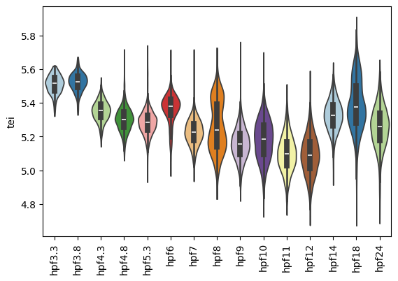
Once the gene age data has been added to the scRNA dataset, one can e.g. plot the corresponding transcriptome evolutionary index (TEI) values by any given observation pre-defined in the scRNA dataset.

Boxplot gene age class per embryo stage

[9]:

sc.pl.violin(adata=zebrafish_data,
             keys=['tei'],
             groupby='stage',
             rotation=90,
             palette='Paired',
             stripplot=False,
             inner='box',
             hue='stage',
             legend=False)

calculate bootstrap on subet of the data

[10]:

# calculate bootstrap
orthomap2tei.get_tei(adata=zebrafish_data_subset,
    gene_id=query_orthomap['geneID'],
    gene_age=query_orthomap['PSnum'],
    keep='min',
    layer=None,
    add_var=True,
    var_name='Phylostrata',
    add_obs=True,
    obs_name='tei',
    boot=True,
    bt=10,
    normalize_total=True,
    log1p=True,
    target_sum=1e6,
    chunk_size=100000)

|████████████████████████████████████████| 10/10 [100%] in 2.5s (4.00/s)

[10]:

(                                        tei
 hpf3.3_ZFHIGH_WT_DS5_AAAAGTTGCCTC  5.514485
 hpf3.3_ZFHIGH_WT_DS5_AAACAAGTGTAT  5.503633
 hpf3.3_ZFHIGH_WT_DS5_AAACACCTCGTC  5.488072
 hpf3.3_ZFHIGH_WT_DS5_AAATGAGGTTTN   5.50889
 hpf3.3_ZFHIGH_WT_DS5_AACCCTCTCGAT  5.574979
 ...                                     ...
 hpf4.3_ZFDOME_WT_DS5_CGGACCGCAGGT  5.301656
 hpf4.3_ZFDOME_WT_DS5_CGGATGGCCACT  5.358101
 hpf4.3_ZFDOME_WT_DS5_CGGCAATGCTTG  5.322054
 hpf4.3_ZFDOME_WT_DS5_CGGCAGTGTTAC  5.351171
 hpf4.3_ZFDOME_WT_DS5_CGGCCAGCGGAN  5.402065

 [1000 rows x 1 columns],
                                      boot_0    boot_1    boot_2    boot_3  \
 hpf3.3_ZFHIGH_WT_DS5_AAAAGTTGCCTC  6.759911  6.647228  6.694393  6.849195
 hpf3.3_ZFHIGH_WT_DS5_AAACAAGTGTAT   6.64466  6.624946  6.689043  6.722857
 hpf3.3_ZFHIGH_WT_DS5_AAACACCTCGTC  6.689828  6.718553  6.771587  6.837948
 hpf3.3_ZFHIGH_WT_DS5_AAATGAGGTTTN   6.78249  6.682479  6.687551  6.839673
 hpf3.3_ZFHIGH_WT_DS5_AACCCTCTCGAT  6.705242  6.738627  6.700644  6.805124
 ...                                     ...       ...       ...       ...
 hpf4.3_ZFDOME_WT_DS5_CGGACCGCAGGT  6.702291  6.733482  6.642275  6.853466
 hpf4.3_ZFDOME_WT_DS5_CGGATGGCCACT   6.77451   6.70771  6.707631  6.725549
 hpf4.3_ZFDOME_WT_DS5_CGGCAATGCTTG  6.940786  6.586875  6.724755  6.693181
 hpf4.3_ZFDOME_WT_DS5_CGGCAGTGTTAC  6.753914   6.69377  6.788657  6.836734
 hpf4.3_ZFDOME_WT_DS5_CGGCCAGCGGAN  6.715839  6.721093  6.690696  6.734315

                                      boot_4    boot_5    boot_6    boot_7  \
 hpf3.3_ZFHIGH_WT_DS5_AAAAGTTGCCTC  6.806379  6.684169  6.647911  6.745181
 hpf3.3_ZFHIGH_WT_DS5_AAACAAGTGTAT  6.874048  6.857684  6.640579  6.835806
 hpf3.3_ZFHIGH_WT_DS5_AAACACCTCGTC  6.781303  6.572003  6.632616   6.76269
 hpf3.3_ZFHIGH_WT_DS5_AAATGAGGTTTN  6.712307  6.724935  6.642234   6.80512
 hpf3.3_ZFHIGH_WT_DS5_AACCCTCTCGAT  6.809793   6.68517  6.684571  6.724404
 ...                                     ...       ...       ...       ...
 hpf4.3_ZFDOME_WT_DS5_CGGACCGCAGGT  6.739432  6.761997  6.659034  6.740662
 hpf4.3_ZFDOME_WT_DS5_CGGATGGCCACT  6.792971  6.753959  6.727792  6.888245
 hpf4.3_ZFDOME_WT_DS5_CGGCAATGCTTG  6.728347  6.707649  6.727023  6.785233
 hpf4.3_ZFDOME_WT_DS5_CGGCAGTGTTAC  6.904999  6.758114  6.599089  6.737372
 hpf4.3_ZFDOME_WT_DS5_CGGCCAGCGGAN  6.763937  6.733328  6.556272   6.80844

                                      boot_8    boot_9
 hpf3.3_ZFHIGH_WT_DS5_AAAAGTTGCCTC  6.778171  6.647924
 hpf3.3_ZFHIGH_WT_DS5_AAACAAGTGTAT  6.779376  6.633174
 hpf3.3_ZFHIGH_WT_DS5_AAACACCTCGTC  6.703302  6.685941
 hpf3.3_ZFHIGH_WT_DS5_AAATGAGGTTTN  6.713637  6.626618
 hpf3.3_ZFHIGH_WT_DS5_AACCCTCTCGAT  6.736239  6.686084
 ...                                     ...       ...
 hpf4.3_ZFDOME_WT_DS5_CGGACCGCAGGT  6.550693  6.772745
 hpf4.3_ZFDOME_WT_DS5_CGGATGGCCACT  6.587417   6.79228
 hpf4.3_ZFDOME_WT_DS5_CGGCAATGCTTG  6.635318  6.615079
 hpf4.3_ZFDOME_WT_DS5_CGGCAGTGTTAC  6.828364  6.599813
 hpf4.3_ZFDOME_WT_DS5_CGGCCAGCGGAN  6.743372  6.586846

 [1000 rows x 10 columns])

Please have a look at the documentation of Downstream analysis to get further insides.