oggmap: Step 4 - other evolutionary indices

This notebook will demonstrate how to to add a other evolutionary indices to scRNA data.

Notebook file

Notebook file can be obtained here:

https://raw.githubusercontent.com/kullrich/oggmap/main/docs/notebooks/evolutionary_indices.ipynb

Import libraries

import numpy as np
import pandas as pd
import scanpy as sc
import seaborn as sns
import matplotlib.pyplot as plt
from statannot import add_stat_annotation
# increase dpi
%matplotlib inline
#plt.rcParams['figure.dpi'] = 300
#plt.rcParams['savefig.dpi'] = 300
plt.rcParams['figure.figsize'] = [6, 4.5]
#plt.rcParams['figure.figsize'] = [4.4, 3.3]

Import oggmap python package submodules

# import submodules
from oggmap import qlin, gtf2t2g, of2orthomap, orthomap2tei, datasets, ncbitax

Step 0, Step 1, Step 2 and Step 3

In order to come to Step 4, TEI calculation, one needs to have the results from Step 0, Step 1, Step 2 and Step 3.

The query species in this part is: Caenorhabditis elegans (nematode).

Note: In this tutorial Step 0 and Step 2 are different since other evolutionary indices will be used to weight gene expression. It does not need to be a gene age class but can be any discrete or continuous gene based measurement.

Other evolutionary indices can be e.g.:

• Tajima’sD

• Nucleotide diversity (within species)

• Nucleotide divergence (between species)

• F-statistics

Please have a look at the documentation of Step 0 - run OrthoFinder to get to know what information and files are mandatory to extract gene age classes from OrthoFinder results.

In Step 1 - get taxonomic information you have already been introduced how to extract query lineage information with oggmap and the qlin.get_qlin() function.

In Step 2 - gene age class assignment you have already been introduced how to extract an orthomap (gene age class) from OrthoFinder results with oggmap and the of2orthomap.get_orthomap() function or how to import pre-calculated orthomaps with the orthomap2tei.read_orthomap() function.

In Step 3 - map gene/transcript IDs you have already been introduced how to extract gene IDs from GTF file with orthoamp and the gtf2t2g.parse_gtf() function. You have also been introduced how to use the orthomap2tei.geneset_overlap() function to check the overlap between the gene IDs and have learned how to use the orthomap2tei.replace_by() function to e.g. reduce isoform gene IDs to gene IDs.

Step 0 - Use different pre-calculated evolutionary indices

Diversity parameter were pre-calculated (Ma et al., 2021) and is available here:

https://doi.org/10.5281/zenodo.7242263

or can be accessed with the dataset submodule of oggmap

datasets.ma21_fst(datapath='data') (download folder set to 'data').

datasets.ma21_fst(datapath='data')

100% [..........................................................................] 1049100 / 1049100

'data/Ma2021_Fst.tsv'

Step 1 - get taxonomic information

Please have a look at the documentation of Step 1 - get taxonomic information to get further insides.

# get query species taxonomic lineage information
query_lineage = qlin.get_qlin(q='Caenorhabditis elegans', dbname='data/taxadb.sqlite')

query name: Caenorhabditis elegans
query taxID: 6239
query kingdom: Eukaryota
query lineage names:
['root(1)', 'cellular organisms(131567)', 'Eukaryota(2759)', 'Opisthokonta(33154)', 'Metazoa(33208)', 'Eumetazoa(6072)', 'Bilateria(33213)', 'Protostomia(33317)', 'Ecdysozoa(1206794)', 'Nematoda(6231)', 'Chromadorea(119089)', 'Rhabditida(6236)', 'Rhabditina(2301116)', 'Rhabditomorpha(2301119)', 'Rhabditoidea(55879)', 'Rhabditidae(6243)', 'Peloderinae(55885)', 'Caenorhabditis(6237)', 'Caenorhabditis elegans(6239)']
query lineage:
[1, 131567, 2759, 33154, 33208, 6072, 33213, 33317, 1206794, 6231, 119089, 6236, 2301116, 2301119, 55879, 6243, 55885, 6237, 6239]

Step 2 - gene based measurement (query species evolutionary index)

Here, an other evolutionary index will be used to weight gene expression. It does not need to be a gene age class but can be any discrete or continuous gene based measurement. Continuous values can be binned first and used as gene groups to weigh expression.

Other evolutionary indices can be e.g.:

• Tajima’sD

• Nucleotide diversity (within species)

• Nucleotide divergence (between species)

• F-statistics

# get query species Fst values

# download pre-calculated Fst values here: https://doi.org/10.5281/zenodo.7242263
# or download with datasets.ma21_fst(datapath='data')
query_fst = pd.read_csv('data/Ma2021_Fst.tsv', delimiter='\t')
query_fst

	WormBase_ID	Chr	Gene	TajimaD	NormalizedPi	FayWu	FST
0	WBGene00000001	I	aap-1	-0.6957	0.0002	-1.2575	0.8062
1	WBGene00000002	IV	aat-1	-0.4724	0.0001	-1.4628	0.8846
2	WBGene00000003	V	aat-2	-1.5266	0.0001	0.0816	0.1691
3	WBGene00000004	X	aat-3	-1.6401	0.0003	-4.7685	0.8129
4	WBGene00000005	IV	aat-4	-1.2137	0.0006	-0.7617	0.3725
...	...	...	...	...	...	...	...
20217	WBGene00271701	X	F10D7.10	-0.7428	0.0000	-1.9308	0.1111
20218	WBGene00271703	III	ZK1010.12	-1.3386	0.0008	-3.2528	0.7683
20219	WBGene00271706	II	D2089.8	-0.8312	0.0012	0.4489	0.5551
20220	WBGene00271707	V	ZK105.14	-1.0748	0.0004	-3.2069	0.6433
20221	WBGene00271715	III	B0244.17	-0.6617	0.0010	-1.1870	0.6556

20222 rows × 7 columns

Group evolutionary indices into bins

# see here for additional quantile methods: https://numpy.org/doc/stable/reference/generated/numpy.nanquantile.html

orthomap2tei.get_bins(tobin_df=query_fst,
                      bincol='TajimaD',
                      q=[.1, .2, .3, .4, .5, .6, .7, .8, .9],
                      method='median_unbiased')
orthomap2tei.get_bins(tobin_df=query_fst,
                      bincol='NormalizedPi',
                      q=[.2, .4, .6, .8],
                      method='median_unbiased')
orthomap2tei.get_bins(tobin_df=query_fst,
                      bincol='FayWu',
                      q=[.1, .2, .3, .4, .5, .6, .7, .8, .9],
                      method='median_unbiased')
orthomap2tei.get_bins(tobin_df=query_fst,
                      bincol='FST',
                      q=[.2, .4, .6, .8],
                      method='median_unbiased')

	WormBase_ID	Chr	Gene	TajimaD	NormalizedPi	FayWu	FST	TajimaD_binned	TajimaD_bins	NormalizedPi_binned	NormalizedPi_bins	FayWu_binned	FayWu_bins	FST_binned	FST_bins
0	WBGene00000001	I	aap-1	-0.6957	0.0002	-1.2575	0.8062	8.0	-0.84 >= x < -0.67368	3.0	0.0002 >= x < 0.0004	5.0	-1.68402 >= x < -0.99135	5.0	0.6286 < x
1	WBGene00000002	IV	aat-1	-0.4724	0.0001	-1.4628	0.8846	9.0	-0.67368 >= x < -0.20841999999999972	2.0	0.0001 >= x < 0.0002	5.0	-1.68402 >= x < -0.99135	5.0	0.6286 < x
2	WBGene00000003	V	aat-2	-1.5266	0.0001	0.0816	0.1691	3.0	-1.6187 >= x < -1.4602466666666667	2.0	0.0001 >= x < 0.0002	8.0	0.03219333333333343 >= x < 0.10182000000000008	3.0	0.1347 >= x < 0.3595
3	WBGene00000004	X	aat-3	-1.6401	0.0003	-4.7685	0.8129	2.0	-1.8383 >= x < -1.6187	3.0	0.0002 >= x < 0.0004	2.0	-9.455993333333332 >= x < -3.9512999999999994	5.0	0.6286 < x
4	WBGene00000005	IV	aat-4	-1.2137	0.0006	-0.7617	0.3725	5.0	-1.3196 >= x < -1.1656	4.0	0.0004 >= x < 0.0011	6.0	-0.99135 >= x < 0.0	4.0	0.3595 >= x < 0.6286
...	...	...	...	...	...	...	...	...	...	...	...	...	...	...	...
20217	WBGene00271701	X	F10D7.10	-0.7428	0.0000	-1.9308	0.1111	8.0	-0.84 >= x < -0.67368	1.0	x < 0.0001	4.0	-2.277410000000001 >= x < -1.68402	2.0	0.0 >= x < 0.1347
20218	WBGene00271703	III	ZK1010.12	-1.3386	0.0008	-3.2528	0.7683	4.0	-1.4602466666666667 >= x < -1.3196	4.0	0.0004 >= x < 0.0011	3.0	-3.9512999999999994 >= x < -2.277410000000001	5.0	0.6286 < x
20219	WBGene00271706	II	D2089.8	-0.8312	0.0012	0.4489	0.5551	8.0	-0.84 >= x < -0.67368	5.0	0.0011 < x	10.0	0.2674900000000009 < x	4.0	0.3595 >= x < 0.6286
20220	WBGene00271707	V	ZK105.14	-1.0748	0.0004	-3.2069	0.6433	6.0	-1.1656 >= x < -1.0416	4.0	0.0004 >= x < 0.0011	3.0	-3.9512999999999994 >= x < -2.277410000000001	5.0	0.6286 < x
20221	WBGene00271715	III	B0244.17	-0.6617	0.0010	-1.1870	0.6556	9.0	-0.67368 >= x < -0.20841999999999972	4.0	0.0004 >= x < 0.0011	5.0	-1.68402 >= x < -0.99135	5.0	0.6286 < x

20222 rows × 15 columns

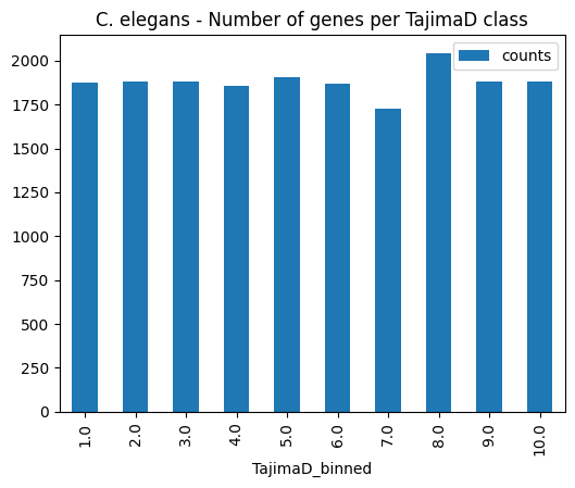
Gene assignments per query species evolutionary index

Given an orthomap, one can get an overview of the gene assignments per query species lineage node.

The oggmap submodule of2orhomap and the of2orthomap.get_counts_per_ps() function will show the distribution of the gene age classes and can be further visualized as follows:

# show count per TajimaD group (TajimaD_binned)
of2orthomap.get_counts_per_ps(omap_df=query_fst,
    psnum_col='TajimaD_binned',
    pstaxid_col=None,
    psname_col=None)

# bar plot count per taxonomic group (PSname)
ax = of2orthomap.get_counts_per_ps(omap_df=query_fst,
    psnum_col='TajimaD_binned',
    pstaxid_col=None,
    psname_col=None).plot.bar(y='counts', x='TajimaD_binned')
ax.set_title('C. elegans - Number of genes per TajimaD class')
plt.show()

Step 3 - map OrthoFinder gene names and scRNA gene/transcript names

To be able to link gene ages assignments from an orthomap and gene or transcript of scRNA dataset, one needs to check the overlap of the annotated gene names. With the gtf2t2g submodule of oggmap and the gtf2t2g.parse_gtf() function, one can extract gene and transcript names from a given gene feature file (GTF).

If in your case gene or transcript IDs between an orthomap and scRNA data do not match directly, please have a look at a detailed how-to to match them:

https://oggmap.readthedocs.io/en/latest/tutorials/geneset_overlap.html

Here, pre-calculated diversity parameter gene names already overlap, so no GTF import is necessary (Ma et al., 2021).

Import now, the scRNA dataset of the query species

Here, data is used, like in the publication (Packer and Zhu al., 2019).

scRNA data was downloaded from https://www.ncbi.nlm.nih.gov/geo/query/acc.cgi?acc=GSE126954 converted into Seurat object and converted into loom and AnnData (h5ad) files to be able to analyse with e.g. python scanpy or oggmap package and is available here:

https://doi.org/10.5281/zenodo.7245547

or can be accessed with the dataset submodule of oggmap:

datasets.packer19(datapath='data') (download folder set to 'data').

Note: A smaller scRNA data set for the same data exist and can be obtained via:

datasets.packer19_small(datapath='data') (download folder set to 'data').

# load scRNA data

# download zebrafish scRNA data here: https://doi.org/10.5281/zenodo.7245547
# or download with datasets.packer19(datapath='data')

#celegans_data = datasets.packer19(datapath='data')
celegans_data = sc.read('data/GSE126954.h5ad')

Get an overview of observations

celegans_data

AnnData object with n_obs × n_vars = 89701 × 20222
    obs: 'orig.ident', 'nCount_RNA', 'nFeature_RNA', 'cell', 'n.umi', 'time.point', 'batch', 'Size_Factor', 'cell.type', 'cell.subtype', 'plot.cell.type', 'raw.embryo.time', 'embryo.time', 'embryo.time.bin', 'raw.embryo.time.bin', 'lineage', 'passed_initial_QC_or_later_whitelisted'
    var: 'features', 'genes'

celegans_data.obs

	orig.ident	nCount_RNA	nFeature_RNA	cell	n.umi	time.point	batch	Size_Factor	cell.type	cell.subtype	plot.cell.type	raw.embryo.time	embryo.time	embryo.time.bin	raw.embryo.time.bin	lineage	passed_initial_QC_or_later_whitelisted
AAACCTGAGACAATAC-300.1.1	0	1630.0	781	AAACCTGAGACAATAC-300.1.1	1630	300_minutes	Waterston_300_minutes	1.023195	Body_wall_muscle	BWM_head_row_1	BWM_head_row_1	360	380.0	330-390	330-390	MSxpappp	1
AAACCTGAGGGCTCTC-300.1.1	0	2323.0	1116	AAACCTGAGGGCTCTC-300.1.1	2319	300_minutes	Waterston_300_minutes	1.458210	NA	NA	NA	260	220.0	210-270	210-270	MSxapaap	1
AAACCTGAGTGCGTGA-300.1.1	0	3725.0	1322	AAACCTGAGTGCGTGA-300.1.1	3719	300_minutes	Waterston_300_minutes	2.338283	NA	NA	NA	270	230.0	210-270	270-330	NA	1
AAACCTGAGTTGAGTA-300.1.1	0	4236.0	1747	AAACCTGAGTTGAGTA-300.1.1	4251	300_minutes	Waterston_300_minutes	2.659051	Body_wall_muscle	BWM_anterior	BWM_anterior	260	280.0	270-330	210-270	Dxap	1
AAACCTGCAAGACGTG-300.1.1	0	1003.0	621	AAACCTGCAAGACGTG-300.1.1	1003	300_minutes	Waterston_300_minutes	0.629610	Ciliated_amphid_neuron	AFD	AFD	350	350.0	330-390	330-390	ABalpppapav/ABpraaaapav	1
...	...	...	...	...	...	...	...	...	...	...	...	...	...	...	...	...	...
TCTGAGACATGTCGAT-b02	0	581.0	361	TCTGAGACATGTCGAT-b02	585	mixed	Murray_b02	0.364709	Rectal_gland	Rectal_gland	Rectal_gland	390	700.0	> 650	390-450	NA	1
TCTGAGACATGTCTCC-b02	0	516.0	327	TCTGAGACATGTCTCC-b02	510	mixed	Murray_b02	0.323907	NA	NA	NA	510	470.0	450-510	510-580	NA	1
TGGCCAGCACGAAGCA-b02	0	843.0	543	TGGCCAGCACGAAGCA-b02	843	mixed	Murray_b02	0.529174	NA	NA	NA	400	470.0	450-510	390-450	NA	1
TGGCGCACAGGCAGTA-b02	0	634.0	397	TGGCGCACAGGCAGTA-b02	636	mixed	Murray_b02	0.397979	NA	NA	NA	330	350.0	330-390	330-390	NA	1
TGGGCGTTCAGGCCCA-b02	0	1126.0	702	TGGGCGTTCAGGCCCA-b02	1132	mixed	Murray_b02	0.706820	NA	NA	NA	260	265.0	210-270	210-270	NA	1

89701 rows × 17 columns

celegans_data.obs.dtypes

orig.ident                                   int32
nCount_RNA                                 float64
nFeature_RNA                                 int32
cell                                        object
n.umi                                        int32
time.point                                category
batch                                     category
Size_Factor                                float64
cell.type                                 category
cell.subtype                              category
plot.cell.type                            category
raw.embryo.time                              int32
embryo.time                                float64
embryo.time.bin                           category
raw.embryo.time.bin                       category
lineage                                   category
passed_initial_QC_or_later_whitelisted       int32
dtype: object

Prior any analysis the observations 'embryo.time.bin' and 'batch' will be converted into the 'category' type. In addition a new observation 'cell.type.per.embryo.time.bin.cat' will be created that combines sample timepoint and assigned cell type.

# add embryo.time.bin as category
celegans_data.obs['embryo.time.bin.cat'] = celegans_data.obs['embryo.time.bin'].astype('category')
celegans_data.obs['embryo.time.bin.cat'] = celegans_data.obs['embryo.time.bin.cat'].cat.reorder_categories(['< 100',
    '100-130','130-170','170-210','210-270','270-330','330-390','390-450','450-510','510-580','580-650','> 650'])
celegans_data.obs['batch.cat'] = celegans_data.obs['batch'].astype('category')

celegans_data.obs['cell.type.per.embryo.time.bin.cat'] =\
    (celegans_data.obs['cell.type'].astype('string') +\
    '-' +\
    celegans_data.obs['embryo.time.bin.cat'].astype('string')).astype('category')

Helper functions to match gene names

The orthomap2tei submodule contains the orthomap2tei.geneset_overlap() helper function to check for gene name overlap between the constructed orthomap from OrthoFinder results and a given scRNA dataset.

# check overlap of orthomap <seqID> and scRNA data <var_names>
orthomap2tei.geneset_overlap(celegans_data.var_names, query_fst['WormBase_ID'])

	g1_g2_overlap	g1_ratio	g2_ratio
0	20222	1.0	1.0

Step 4 - Get TEI values and add them to scRNA dataset

Since now the gene names correspond to each other in the orthomap and the scRNA adata object, one can calculate the transcriptome evolutionary index (TEI) and add them to the scRNA dataset (adata object).

The TEI measure represents the weighted arithmetic mean (expression levels as weights for the gene based measurement) over all categories.

\({TEI_s = \sum (e_{is} * m_i) / \sum e_{is}}\)

, where \({TEI_s}\) denotes the TEI value in developmental stage \({s, e_{is}}\) denotes the gene expression level of gene \({i}\) in stage \({s}\), and \({m_i}\) denotes the corresponding measurement of gene \({i, i = 1,...,N}\) and \({N = total\ number\ of\ genes}\).

Note: If e.g. two different isoforms would fall into two different categories, their gene measurement might differ based on the underlying calculation. However, both isoforms share the same gene name and their gene measurement would clash. In this case one can decide either to use the keep='min' or keep='max' gene measurement to be kept by the get_tei function, which defaults to keep in this cases the keep='min' or in other words the ‘minimal’ gene measurement.

To be able to re-use the original count data, they are added as a new layer to the adata object. This is useful because later on the count data can be used to extract either the relative expression per gene age class or re-calculate other metrics.

This can be done either on un-normalized counts, on normalized and log-transformed data.

celegans_data.layers['counts'] = celegans_data.X

add TEI to adata object

Using the submodule orthomap2tei from oggmap and the orthomap2tei.get_tei() function, transcriptome evolutionary index (TEI) values are calculated and directyl added to the existing adata object (add_obs=True).

There are other options to e.g. not start from the adata.X counts but from another layer from the adata object, the default is to use the adata.X (layer=None). The values can be pre-processed by the normalize_total option and the log1p option.

If add_obs=True the resulting TEI values are added to the existing adata object as a new observation with the name set with the obs_name option.

If add_var=True the gene age values are added to the existing adata object as a new variable with the name set with the var_name option.

Note: Genes not assigned to any gene class will get a missing assignment.

If one wants to calculate bootstrap TEI values per cell, the boot option can be set to boot=True and gene age classes will be randomly chosen prior calculating TEI values bt=10 times.

add TajimaD, Fst and NormalizedPi to adata object

# add TajimaD binned values to existing adata object
orthomap2tei.get_tei(adata=celegans_data,
    gene_id=query_fst['WormBase_ID'],
    gene_age=query_fst['TajimaD_binned'],
    keep='min',
    layer=None,
    add_var=True,
    var_name='TajimaD_bin',
    add_obs=True,
    obs_name='TajimaD',
    boot=False,
    bt=10,
    normalize_total=True,
    log1p=True,
    target_sum=1e6)

	TajimaD
AAACCTGAGACAATAC-300.1.1	5.769133
AAACCTGAGGGCTCTC-300.1.1	5.898489
AAACCTGAGTGCGTGA-300.1.1	5.736505
AAACCTGAGTTGAGTA-300.1.1	5.795881
AAACCTGCAAGACGTG-300.1.1	5.746057
...	...
TCTGAGACATGTCGAT-b02	5.465485
TCTGAGACATGTCTCC-b02	5.543912
TGGCCAGCACGAAGCA-b02	5.524013
TGGCGCACAGGCAGTA-b02	5.652469
TGGGCGTTCAGGCCCA-b02	5.634361

89701 rows × 1 columns

# add Fst binned values to existing adata object
orthomap2tei.get_tei(adata=celegans_data,
    gene_id=query_fst['WormBase_ID'],
    gene_age=query_fst['FST_binned'],
    keep='min',
    layer=None,
    add_var=True,
    var_name='FST_bin',
    add_obs=True,
    obs_name='Fst',
    boot=False,
    bt=10,
    normalize_total=True,
    log1p=True,
    target_sum=1e6)

	Fst
AAACCTGAGACAATAC-300.1.1	2.997840
AAACCTGAGGGCTCTC-300.1.1	3.103704
AAACCTGAGTGCGTGA-300.1.1	3.100244
AAACCTGAGTTGAGTA-300.1.1	3.105081
AAACCTGCAAGACGTG-300.1.1	3.011721
...	...
TCTGAGACATGTCGAT-b02	3.011302
TCTGAGACATGTCTCC-b02	3.134352
TGGCCAGCACGAAGCA-b02	3.054067
TGGCGCACAGGCAGTA-b02	3.117862
TGGGCGTTCAGGCCCA-b02	3.149005

89701 rows × 1 columns

# add NormalizedPi binned values to existing adata object
orthomap2tei.get_tei(adata=celegans_data,
    gene_id=query_fst['WormBase_ID'],
    gene_age=query_fst['NormalizedPi_binned'],
    keep='min',
    layer=None,
    add_var=True,
    var_name='NormalizedPi_bin',
    add_obs=True,
    obs_name='NormalizedPi',
    boot=False,
    bt=10,
    normalize_total=True,
    log1p=True,
    target_sum=1e6)

	NormalizedPi
AAACCTGAGACAATAC-300.1.1	2.321107
AAACCTGAGGGCTCTC-300.1.1	2.527517
AAACCTGAGTGCGTGA-300.1.1	2.445354
AAACCTGAGTTGAGTA-300.1.1	2.507382
AAACCTGCAAGACGTG-300.1.1	2.655676
...	...
TCTGAGACATGTCGAT-b02	2.267350
TCTGAGACATGTCTCC-b02	2.484896
TGGCCAGCACGAAGCA-b02	2.378922
TGGCGCACAGGCAGTA-b02	2.483049
TGGGCGTTCAGGCCCA-b02	2.470968

89701 rows × 1 columns

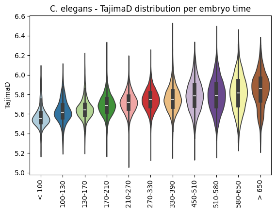
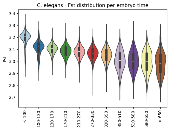
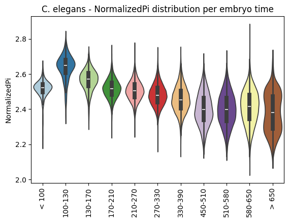
Step 5 - downstream analysis

Once the gene age data has been added to the scRNA dataset, one can e.g. plot the corresponding transcriptome evolutionary index (TEI) values by any given observation pre-defined in the scRNA dataset.

Here, we plot them against the assigned embryo stage and against assigned cell types of the zebrafish using the scanpy sc.pl.violin() function as follows:

Boxplot TajimaD class per sample timepoint

ax = sc.pl.violin(adata=celegans_data,
                  keys=['TajimaD'],
                  groupby='embryo.time.bin.cat',
                  rotation=90,
                  palette='Paired',
                  stripplot=False,
                  inner='box',
                  order=['< 100', '100-130', '130-170', '170-210',
                         '210-270', '270-330', '330-390', '450-510',
                         '510-580', '580-650', '> 650'],
                  show=False,
                  hue='embryo.time.bin.cat',
                  legend=False)
ax.set_title('C. elegans - TajimaD distribution per embryo time')
plt.show()

Boxplot Fst class per sample timepoint

ax = sc.pl.violin(adata=celegans_data,
                  keys=['Fst'],
                  groupby='embryo.time.bin.cat',
                  rotation=90,
                  palette='Paired',
                  stripplot=False,
                  inner='box',
                  order=['< 100', '100-130', '130-170', '170-210',
                         '210-270', '270-330', '330-390', '450-510',
                         '510-580', '580-650', '> 650'],
                  show=False,
                  hue='embryo.time.bin.cat',
                  legend=False)
ax.set_title('C. elegans - Fst distribution per embryo time')
plt.show()

Boxplot NormalizedPi class per sample timepoint

ax = sc.pl.violin(adata=celegans_data,
                  keys=['NormalizedPi'],
                  groupby='embryo.time.bin.cat',
                  rotation=90,
                  palette='Paired',
                  stripplot=False,
                  inner='box',
                  order=['< 100', '100-130', '130-170', '170-210',
                         '210-270', '270-330', '330-390', '450-510',
                         '510-580', '580-650', '> 650'],
                  show=False,
                  hue='embryo.time.bin.cat',
                  legend=False)
ax.set_title('C. elegans - NormalizedPi distribution per embryo time')
plt.show()

Please have a look at the documentation of the nematode example to see more downstream analysis e.g. how to compare gene age and other evolutionary indices of the same scRNA data or have a look at the documentation for other case studies.