Case study: re-analysis of nematode (Caenorhabditis elegans) embryogenesis single-cell data

This notebook will demonstrate scRNA-seq processing with oggmap using nematode scRNA data from (Packer and Zhu al., 2019).

scRNA data were obtained from https://www.ncbi.nlm.nih.gov/geo/query/acc.cgi?acc=GSE126954, converted into Scanpy AnnData objects (Wolf et al., 2018) and are availabe here:

https://doi.org/10.5281/zenodo.7245547

or can be accessed with the dataset submodule of oggmap

datasets.packer19(datapath='data') (download folder set to 'data').

Notebook file

Notebook file can be obtained here:

https://raw.githubusercontent.com/kullrich/oggmap/main/docs/notebooks/nematode_example.ipynb

Steps

To process the scRNA data, we will do the following:

Use pre-calculated gene age classification
Get query species taxonomic lineage information
Get query species orthomap
Map OrthoFinder gene names and scRNA gene/transcript names
Get TEI values and add them to scRNA dataset
Get partial TEI values to visualize gene age class contributions
Process scRNA data and visualize TEI

Import libraries

[1]:

import numpy as np
import pandas as pd
import scanpy as sc
import seaborn as sns
import matplotlib.pyplot as plt
from statannot import add_stat_annotation
# increase dpi
%matplotlib inline
#plt.rcParams['figure.dpi'] = 300
#plt.rcParams['savefig.dpi'] = 300
#plt.rcParams['figure.figsize'] = [6, 4.5]
plt.rcParams['figure.figsize'] = [4.4, 3.3]

Import oggmap python package submodules

[2]:

# import submodules
from oggmap import qlin, gtf2t2g, of2orthomap, orthomap2tei, datasets

Step 0 - Use pre-calculated gene age classification

Orthomap was pre-calculated (Sun et al., 2021) and is available here:

https://doi.org/10.5281/zenodo.7242263

or can be accessed with the dataset submodule of oggmap

datasets.sun21_orthomap(datapath='data') (download folder set to 'data').

If you want to use your own OrthoFinder results:

oggmap can extract gene age classification from existing OrthoFinder results and link them with scRNA data.

A detailed how-to is available here:

https://oggmap.readthedocs.io/en/latest/tutorials/orthofinder.html

[3]:

# download pre-calculated orthomap into data folder
datasets.sun21_orthomap(datapath='data')

100% [........................................................] 344640 / 344640

[3]:

'data/Sun2021_Orthomap.tsv'

Step 0 - Use different pre-calculated evolutionary indices

Diversity parameter were pre-calculated (Ma et al., 2021) and is available here:

https://doi.org/10.5281/zenodo.7242263

or can be accessed with the dataset submodule of oggmap

datasets.ma21_orthomap(datapath='data') (download folder set to 'data').

[4]:

# download pre-calculated evolutionay indices into data folder
datasets.ma21_fst(datapath='data')

100% [......................................................] 1049100 / 1049100

[4]:

'data/Ma2021_Fst.tsv'

Step 1 - get query species taxonomic lineage information

Given a species name or taxonomic ID, the query species lineage information is extracted with the help of the ete3 python toolkit and the NCBI taxonomy (Huerta-Cepas et al., 2016). This information is needed alongside with the taxonomic classifications for all species used in the OrthoFinder comparison.

The oggmap submodule qlin helps to get this information for you with the qlin.get_qlin() function as follows:

[5]:

# get query species taxonomic lineage information
query_lineage = qlin.get_qlin(q='Caenorhabditis elegans')

query name: Caenorhabditis elegans
query taxID: 6239
query kingdom: Eukaryota
query lineage names:
['root(1)', 'cellular organisms(131567)', 'Eukaryota(2759)', 'Opisthokonta(33154)', 'Metazoa(33208)', 'Eumetazoa(6072)', 'Bilateria(33213)', 'Protostomia(33317)', 'Ecdysozoa(1206794)', 'Nematoda(6231)', 'Chromadorea(119089)', 'Rhabditida(6236)', 'Rhabditina(2301116)', 'Rhabditomorpha(2301119)', 'Rhabditoidea(55879)', 'Rhabditidae(6243)', 'Peloderinae(55885)', 'Caenorhabditis(6237)', 'Caenorhabditis elegans(6239)']
query lineage:
[1, 131567, 2759, 33154, 33208, 6072, 33213, 33317, 1206794, 6231, 119089, 6236, 2301116, 2301119, 55879, 6243, 55885, 6237, 6239]

Step 2 - gene age class assignment (query species orthomap)

Orthomap was pre-calculated (Sun et al., 2021; see Figure 3B) it is also available here:

https://doi.org/10.5281/zenodo.7242263

or can be accessed with the dataset submodule of oggmap

datasets.sun21_orthomap(datapath='data') (download folder set to 'data').

The pre-calculated orthomap can be imported from the orthomap2tei submodule with the orthomap2tei.read_orthomap() function as follwos:

[6]:

# get query species orthomap

# download pre-calculated orthomap here: https://doi.org/10.5281/zenodo.7242263
# or download with datasets.sun21_orthomap(datapath='data')
query_orthomap = orthomap2tei.read_orthomap(orthomapfile='data/Sun2021_Orthomap.tsv')
query_orthomap

[6]:

	GeneID	Phylostratum
0	WBGene00000001	1
1	WBGene00000002	1
2	WBGene00000003	1
3	WBGene00000004	1
4	WBGene00000005	2
...	...	...
20035	WBGene00305132	9
20036	WBGene00305157	1
20037	WBGene00305158	13
20038	WBGene00305159	11
20039	WBGene00305173	0

20040 rows × 2 columns

Get query species evolutionary indices

[7]:

# get query species Fst values

# download pre-calculated Fst values here: https://doi.org/10.5281/zenodo.7242263
# or download with datasets.ma21_fst(datapath='data')
query_fst = pd.read_csv('data/Ma2021_Fst.tsv', delimiter='\t')
query_fst

[7]:

	WormBase_ID	Chr	Gene	TajimaD	NormalizedPi	FayWu	FST
0	WBGene00000001	I	aap-1	-0.6957	0.0002	-1.2575	0.8062
1	WBGene00000002	IV	aat-1	-0.4724	0.0001	-1.4628	0.8846
2	WBGene00000003	V	aat-2	-1.5266	0.0001	0.0816	0.1691
3	WBGene00000004	X	aat-3	-1.6401	0.0003	-4.7685	0.8129
4	WBGene00000005	IV	aat-4	-1.2137	0.0006	-0.7617	0.3725
...	...	...	...	...	...	...	...
20217	WBGene00271701	X	F10D7.10	-0.7428	0.0000	-1.9308	0.1111
20218	WBGene00271703	III	ZK1010.12	-1.3386	0.0008	-3.2528	0.7683
20219	WBGene00271706	II	D2089.8	-0.8312	0.0012	0.4489	0.5551
20220	WBGene00271707	V	ZK105.14	-1.0748	0.0004	-3.2069	0.6433
20221	WBGene00271715	III	B0244.17	-0.6617	0.0010	-1.1870	0.6556

20222 rows × 7 columns

Group evolutionary indices into bins

[8]:

# see here for additional quantile methods: https://numpy.org/doc/stable/reference/generated/numpy.nanquantile.html

orthomap2tei.get_bins(tobin_df=query_fst,
                      bincol='TajimaD',
                      q=[.1, .2, .3, .4, .5, .6, .7, .8, .9],
                      method='median_unbiased')
orthomap2tei.get_bins(tobin_df=query_fst,
                      bincol='NormalizedPi',
                      q=[.2, .4, .6, .8],
                      method='median_unbiased')
orthomap2tei.get_bins(tobin_df=query_fst,
                      bincol='FayWu',
                      q=[.1, .2, .3, .4, .5, .6, .7, .8, .9],
                      method='median_unbiased')
orthomap2tei.get_bins(tobin_df=query_fst,
                      bincol='FST',
                      q=[.2, .4, .6, .8],
                      method='median_unbiased')

[8]:

	WormBase_ID	Chr	Gene	TajimaD	NormalizedPi	FayWu	FST	TajimaD_binned	TajimaD_bins	NormalizedPi_binned	NormalizedPi_bins	FayWu_binned	FayWu_bins	FST_binned	FST_bins
0	WBGene00000001	I	aap-1	-0.6957	0.0002	-1.2575	0.8062	8.0	-0.84 >= x < -0.67368	3.0	0.0002 >= x < 0.0004	5.0	-1.68402 >= x < -0.99135	5.0	0.6286 < x
1	WBGene00000002	IV	aat-1	-0.4724	0.0001	-1.4628	0.8846	9.0	-0.67368 >= x < -0.20841999999999972	2.0	0.0001 >= x < 0.0002	5.0	-1.68402 >= x < -0.99135	5.0	0.6286 < x
2	WBGene00000003	V	aat-2	-1.5266	0.0001	0.0816	0.1691	3.0	-1.6187 >= x < -1.4602466666666667	2.0	0.0001 >= x < 0.0002	8.0	0.03219333333333343 >= x < 0.10182000000000008	3.0	0.1347 >= x < 0.3595
3	WBGene00000004	X	aat-3	-1.6401	0.0003	-4.7685	0.8129	2.0	-1.8383 >= x < -1.6187	3.0	0.0002 >= x < 0.0004	2.0	-9.455993333333332 >= x < -3.9512999999999994	5.0	0.6286 < x
4	WBGene00000005	IV	aat-4	-1.2137	0.0006	-0.7617	0.3725	5.0	-1.3196 >= x < -1.1656	4.0	0.0004 >= x < 0.0011	6.0	-0.99135 >= x < 0.0	4.0	0.3595 >= x < 0.6286
...	...	...	...	...	...	...	...	...	...	...	...	...	...	...	...
20217	WBGene00271701	X	F10D7.10	-0.7428	0.0000	-1.9308	0.1111	8.0	-0.84 >= x < -0.67368	1.0	x < 0.0001	4.0	-2.277410000000001 >= x < -1.68402	2.0	0.0 >= x < 0.1347
20218	WBGene00271703	III	ZK1010.12	-1.3386	0.0008	-3.2528	0.7683	4.0	-1.4602466666666667 >= x < -1.3196	4.0	0.0004 >= x < 0.0011	3.0	-3.9512999999999994 >= x < -2.277410000000001	5.0	0.6286 < x
20219	WBGene00271706	II	D2089.8	-0.8312	0.0012	0.4489	0.5551	8.0	-0.84 >= x < -0.67368	5.0	0.0011 < x	10.0	0.2674900000000009 < x	4.0	0.3595 >= x < 0.6286
20220	WBGene00271707	V	ZK105.14	-1.0748	0.0004	-3.2069	0.6433	6.0	-1.1656 >= x < -1.0416	4.0	0.0004 >= x < 0.0011	3.0	-3.9512999999999994 >= x < -2.277410000000001	5.0	0.6286 < x
20221	WBGene00271715	III	B0244.17	-0.6617	0.0010	-1.1870	0.6556	9.0	-0.67368 >= x < -0.20841999999999972	4.0	0.0004 >= x < 0.0011	5.0	-1.68402 >= x < -0.99135	5.0	0.6286 < x

20222 rows × 15 columns

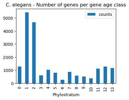
Gene age assignments per query species lineage node

Given an orthomap, one can get an overview of the gene age assignments per query species lineage node.

The oggmap submodule of2orhomap and the of2orthomap.get_counts_per_ps() function will show the distribution of the gene age classes and can be further visualized as follows:

[9]:

# show count per taxonomic group (PStaxID)
of2orthomap.get_counts_per_ps(omap_df=query_orthomap,
    psnum_col='Phylostratum',
    pstaxid_col=None,
    psname_col=None)

# bar plot count per taxonomic group (PSname)
ax = of2orthomap.get_counts_per_ps(omap_df=query_orthomap,
    psnum_col='Phylostratum',
    pstaxid_col=None,
    psname_col=None).plot.bar(y='counts', x='Phylostratum')
ax.set_title('C. elegans - Number of genes per gene age class')
plt.show()

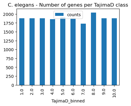
../_images/notebooks_nematode_example_20_0.png

Gene assignments per query species evolutionary index

[10]:

# show count per TajimaD group (TajimaD_binned)
of2orthomap.get_counts_per_ps(omap_df=query_fst,
    psnum_col='TajimaD_binned',
    pstaxid_col=None,
    psname_col=None)

# bar plot count per taxonomic group (PSname)
ax = of2orthomap.get_counts_per_ps(omap_df=query_fst,
    psnum_col='TajimaD_binned',
    pstaxid_col=None,
    psname_col=None).plot.bar(y='counts', x='TajimaD_binned')
ax.set_title('C. elegans - Number of genes per TajimaD class')
plt.show()

../_images/notebooks_nematode_example_22_0.png

Step 3 - map OrthoFinder gene names and scRNA gene/transcript names

To be able to link gene ages assignments from an orthomap and gene or transcript of scRNA dataset, one needs to check the overlap of the annotated gene names. With the gtf2t2g submodule of oggmap and the gtf2t2g.parse_gtf() function, one can extract gene and transcript names from a given gene feature file (GTF).

Here, pre-calculated orthomap gene names already overlap, so no GTF import is necessary (Sun et al., 2021).

Import now, the scRNA dataset of the query species

Here, data is used, like in the original publication (Packer and Zhu al., 2019).

scRNA data were downloaded from https://www.ncbi.nlm.nih.gov/geo/query/acc.cgi?acc=GSE126954 converted into Seurat object and converted into loom and AnnData (h5ad) files to be able to analyse with e.g. python scanpy or oggmap package and is availbale here:

https://doi.org/10.5281/zenodo.7245547

or can be accessed with the dataset submodule of oggmap:

datasets.packer19(datapath='data') (download folder set to 'data').

Note: A smaller scRNA data set for the same data exist and can be obtained via:

datasets.packer19_small(datapath='data') (download folder set to 'data').

[11]:

# load scRNA data

# download zebrafish scRNA data here: https://doi.org/10.5281/zenodo.7245547
# or download with datasets.packer19('data')

#celegans_data = datasets.packer19(datapath='data')
celegans_data = sc.read('data/GSE126954.h5ad')

Get an overview of observations

[12]:

celegans_data

[12]:

AnnData object with n_obs × n_vars = 89701 × 20222
    obs: 'orig.ident', 'nCount_RNA', 'nFeature_RNA', 'cell', 'n.umi', 'time.point', 'batch', 'Size_Factor', 'cell.type', 'cell.subtype', 'plot.cell.type', 'raw.embryo.time', 'embryo.time', 'embryo.time.bin', 'raw.embryo.time.bin', 'lineage', 'passed_initial_QC_or_later_whitelisted'
    var: 'features', 'genes'

[13]:

celegans_data.obs

[13]:

	orig.ident	nCount_RNA	nFeature_RNA	cell	n.umi	time.point	batch	Size_Factor	cell.type	cell.subtype	plot.cell.type	raw.embryo.time	embryo.time	embryo.time.bin	raw.embryo.time.bin	lineage	passed_initial_QC_or_later_whitelisted
AAACCTGAGACAATAC-300.1.1	0	1630.0	781	AAACCTGAGACAATAC-300.1.1	1630	300_minutes	Waterston_300_minutes	1.023195	Body_wall_muscle	BWM_head_row_1	BWM_head_row_1	360	380.0	330-390	330-390	MSxpappp	1
AAACCTGAGGGCTCTC-300.1.1	0	2323.0	1116	AAACCTGAGGGCTCTC-300.1.1	2319	300_minutes	Waterston_300_minutes	1.458210	NA	NA	NA	260	220.0	210-270	210-270	MSxapaap	1
AAACCTGAGTGCGTGA-300.1.1	0	3725.0	1322	AAACCTGAGTGCGTGA-300.1.1	3719	300_minutes	Waterston_300_minutes	2.338283	NA	NA	NA	270	230.0	210-270	270-330	NA	1
AAACCTGAGTTGAGTA-300.1.1	0	4236.0	1747	AAACCTGAGTTGAGTA-300.1.1	4251	300_minutes	Waterston_300_minutes	2.659051	Body_wall_muscle	BWM_anterior	BWM_anterior	260	280.0	270-330	210-270	Dxap	1
AAACCTGCAAGACGTG-300.1.1	0	1003.0	621	AAACCTGCAAGACGTG-300.1.1	1003	300_minutes	Waterston_300_minutes	0.629610	Ciliated_amphid_neuron	AFD	AFD	350	350.0	330-390	330-390	ABalpppapav/ABpraaaapav	1
...	...	...	...	...	...	...	...	...	...	...	...	...	...	...	...	...	...
TCTGAGACATGTCGAT-b02	0	581.0	361	TCTGAGACATGTCGAT-b02	585	mixed	Murray_b02	0.364709	Rectal_gland	Rectal_gland	Rectal_gland	390	700.0	> 650	390-450	NA	1
TCTGAGACATGTCTCC-b02	0	516.0	327	TCTGAGACATGTCTCC-b02	510	mixed	Murray_b02	0.323907	NA	NA	NA	510	470.0	450-510	510-580	NA	1
TGGCCAGCACGAAGCA-b02	0	843.0	543	TGGCCAGCACGAAGCA-b02	843	mixed	Murray_b02	0.529174	NA	NA	NA	400	470.0	450-510	390-450	NA	1
TGGCGCACAGGCAGTA-b02	0	634.0	397	TGGCGCACAGGCAGTA-b02	636	mixed	Murray_b02	0.397979	NA	NA	NA	330	350.0	330-390	330-390	NA	1
TGGGCGTTCAGGCCCA-b02	0	1126.0	702	TGGGCGTTCAGGCCCA-b02	1132	mixed	Murray_b02	0.706820	NA	NA	NA	260	265.0	210-270	210-270	NA	1

89701 rows × 17 columns

[14]:

celegans_data.obs.dtypes

[14]:

orig.ident                                   int32
nCount_RNA                                 float64
nFeature_RNA                                 int32
cell                                        object
n.umi                                        int32
time.point                                category
batch                                     category
Size_Factor                                float64
cell.type                                 category
cell.subtype                              category
plot.cell.type                            category
raw.embryo.time                              int32
embryo.time                                float64
embryo.time.bin                           category
raw.embryo.time.bin                       category
lineage                                   category
passed_initial_QC_or_later_whitelisted       int32
dtype: object

Prior any analysis the observations 'embryo.time.bin' and 'batch' will be converted into the 'category' type. In addition a new observation 'cell.type.per.embryo.time.bin.cat' will be created that combines sample timepoint and assigned cell type.

[15]:

# add embryo.time.bin as category
celegans_data.obs['embryo.time.bin.cat'] = celegans_data.obs['embryo.time.bin'].astype('category')
celegans_data.obs['embryo.time.bin.cat'] = celegans_data.obs['embryo.time.bin.cat'].cat.reorder_categories(['< 100',
    '100-130','130-170','170-210','210-270','270-330','330-390','390-450','450-510','510-580','580-650','> 650'])
celegans_data.obs['batch.cat'] = celegans_data.obs['batch'].astype('category')

[16]:

celegans_data.obs['cell.type.per.embryo.time.bin.cat'] =\
    (celegans_data.obs['cell.type'].astype('string') +\
    '-' +\
    celegans_data.obs['embryo.time.bin.cat'].astype('string')).astype('category')

Helper functions to match gene names

The orthomap2tei submodule contains the orthomap2tei.geneset_overlap() helper function to check for gene name overlap between the constructed orthomap from OrthoFinder results and a given scRNA dataset.

[17]:

# check overlap of orthomap <seqID> and scRNA data <var_names>
orthomap2tei.geneset_overlap(geneset1=celegans_data.var_names,
                             geneset2=query_orthomap['GeneID'])

[17]:

	g1_g2_overlap	g1_ratio	g2_ratio
0	19795	0.978884	0.987774

step 4 - Get TEI values and add them to scRNA dataset

Since now the gene names correspond to each other in the orthomap and the scRNA adata object, one can calculate the transcriptome evolutionary index (TEI) and add them to the scRNA dataset (adata object).

The TEI measure represents the weighted arithmetic mean (expression levels as weights for the phylostratum value) over all evolutionary age categories denoted as phylostra.

\({TEI_s = \sum (e_{is} * ps_i) / \sum e_{is}}\)

, where \({TEI_s}\) denotes the TEI value in developmental stage \({s, e_{is}}\) denotes the gene expression level of gene \({i}\) in stage \({s}\), and \({ps_i}\) denotes the corresponding phylostratum of gene \({i, i = 1,...,N}\) and \({N = total\ number\ of\ genes}\).

Note: If e.g. two different isoforms would fall into two different gene age classes, their gene ages might differ based on the oldest ortholog found in their corresponding orthologous groups. However, both isoforms share the same gene name and their gene ages would clash. In this case one can decide either to use the keep='min' or keep='max' gene age to be kept by the get_tei function, which defaults to keep in this cases the keep='min' or in other words the ‘older’ gene age.

To be able to re-use the original count data, they are added as a new layer to the adata object. This is useful because later on the count data can be used to extract either the relative expression per gene age class.

This can be done either on un-normalized counts, on normalized and log-transformed data.

[18]:

celegans_data.layers['counts'] = celegans_data.X

add TEI to adata object

Using the submodule orthomap2tei from oggmap and the orthomap2tei.get_tei() function, transcriptome evolutionary index (TEI) values are calculated and directyl added to the existing adata object (add_obs=True).

There are other options to e.g. not start from the adata.X counts but from another layer from the adata object, the default is to use the adata.X (layer=None). The values can be pre-processed by the normalize_total option and the log1p option.

If add_obs=True the resulting TEI values are added to the existing adata object as a new observation with the name set with the obs_name option.

If add_var=True the gene age values are added to the existing adata object as a new variable with the name set with the var_name option.

Note: Genes not assigned to any gene class will get a missing assignment.

If one wants to calculate bootstrap TEI values per cell, the boot option can be set to boot=True and gene age classes will be randomly chosen prior calculating TEI values bt=10 times.

[19]:

# add TEI values to existing adata object
orthomap2tei.get_tei(adata=celegans_data,
    gene_id=query_orthomap['GeneID'],
    gene_age=query_orthomap['Phylostratum'],
    keep='min',
    layer=None,
    add_var=True,
    var_name='Phylostrata',
    add_obs=True,
    obs_name='tei',
    boot=False,
    bt=10,
    normalize_total=True,
    log1p=True,
    target_sum=1e6)

[19]:

	tei
AAACCTGAGACAATAC-300.1.1	1.876533
AAACCTGAGGGCTCTC-300.1.1	2.239562
AAACCTGAGTGCGTGA-300.1.1	2.126684
AAACCTGAGTTGAGTA-300.1.1	2.362362
AAACCTGCAAGACGTG-300.1.1	2.581323
...	...
TCTGAGACATGTCGAT-b02	1.964531
TCTGAGACATGTCTCC-b02	2.155930
TGGCCAGCACGAAGCA-b02	2.262958
TGGCGCACAGGCAGTA-b02	2.565133
TGGGCGTTCAGGCCCA-b02	2.269434

89701 rows × 1 columns

add TajimaD, Fst and NormalizedPi to adata object

[20]:

# add TajimaD binned values to existing adata object
orthomap2tei.get_tei(adata=celegans_data,
    gene_id=query_fst['WormBase_ID'],
    gene_age=query_fst['TajimaD_binned'],
    keep='min',
    layer=None,
    add_var=True,
    var_name='TajimaD_bin',
    add_obs=True,
    obs_name='TajimaD',
    boot=False,
    bt=10,
    normalize_total=True,
    log1p=True,
    target_sum=1e6)

[20]:

	TajimaD
AAACCTGAGACAATAC-300.1.1	5.769133
AAACCTGAGGGCTCTC-300.1.1	5.898489
AAACCTGAGTGCGTGA-300.1.1	5.736505
AAACCTGAGTTGAGTA-300.1.1	5.795881
AAACCTGCAAGACGTG-300.1.1	5.746057
...	...
TCTGAGACATGTCGAT-b02	5.465485
TCTGAGACATGTCTCC-b02	5.543912
TGGCCAGCACGAAGCA-b02	5.524013
TGGCGCACAGGCAGTA-b02	5.652469
TGGGCGTTCAGGCCCA-b02	5.634361

89701 rows × 1 columns

[21]:

# add Fst binned values to existing adata object
orthomap2tei.get_tei(adata=celegans_data,
    gene_id=query_fst['WormBase_ID'],
    gene_age=query_fst['FST_binned'],
    keep='min',
    layer=None,
    add_var=True,
    var_name='FST_bin',
    add_obs=True,
    obs_name='Fst',
    boot=False,
    bt=10,
    normalize_total=True,
    log1p=True,
    target_sum=1e6)

[21]:

	Fst
AAACCTGAGACAATAC-300.1.1	2.997840
AAACCTGAGGGCTCTC-300.1.1	3.103704
AAACCTGAGTGCGTGA-300.1.1	3.100244
AAACCTGAGTTGAGTA-300.1.1	3.105081
AAACCTGCAAGACGTG-300.1.1	3.011721
...	...
TCTGAGACATGTCGAT-b02	3.011302
TCTGAGACATGTCTCC-b02	3.134352
TGGCCAGCACGAAGCA-b02	3.054067
TGGCGCACAGGCAGTA-b02	3.117862
TGGGCGTTCAGGCCCA-b02	3.149005

89701 rows × 1 columns

[22]:

# add NormalizedPi binned values to existing adata object
orthomap2tei.get_tei(adata=celegans_data,
    gene_id=query_fst['WormBase_ID'],
    gene_age=query_fst['NormalizedPi_binned'],
    keep='min',
    layer=None,
    add_var=True,
    var_name='NormalizedPi_bin',
    add_obs=True,
    obs_name='NormalizedPi',
    boot=False,
    bt=10,
    normalize_total=True,
    log1p=True,
    target_sum=1e6)

[22]:

	NormalizedPi
AAACCTGAGACAATAC-300.1.1	2.321107
AAACCTGAGGGCTCTC-300.1.1	2.527517
AAACCTGAGTGCGTGA-300.1.1	2.445354
AAACCTGAGTTGAGTA-300.1.1	2.507382
AAACCTGCAAGACGTG-300.1.1	2.655676
...	...
TCTGAGACATGTCGAT-b02	2.267350
TCTGAGACATGTCTCC-b02	2.484896
TGGCCAGCACGAAGCA-b02	2.378922
TGGCGCACAGGCAGTA-b02	2.483049
TGGGCGTTCAGGCCCA-b02	2.470968

89701 rows × 1 columns

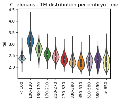
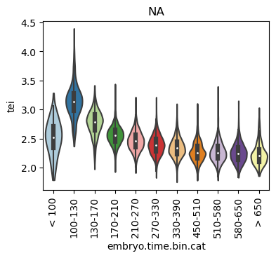
Step 5 - downstream analysis

Once the gene age data has been added to the scRNA dataset, one can e.g. plot the corresponding transcriptome evolutionary index (TEI) values by any given observation pre-defined in the scRNA dataset.

Here, we plot them against the assigned sample timepoint and against assigned cell types of the nematode using the scanpy sc.pl.violin() function as follows:

Boxplot gene age class per sample timepoint

[23]:

ax = sc.pl.violin(adata=celegans_data,
                  keys=['tei'],
                  groupby='embryo.time.bin.cat',
                  rotation=90,
                  palette='Paired',
                  stripplot=False,
                  inner='box',
                  order=['< 100', '100-130', '130-170', '170-210',
                         '210-270', '270-330', '330-390', '450-510',
                         '510-580', '580-650', '> 650'],
                  show=False)
ax.set_title('C. elegans - TEI distribution per embryo time')
plt.show()

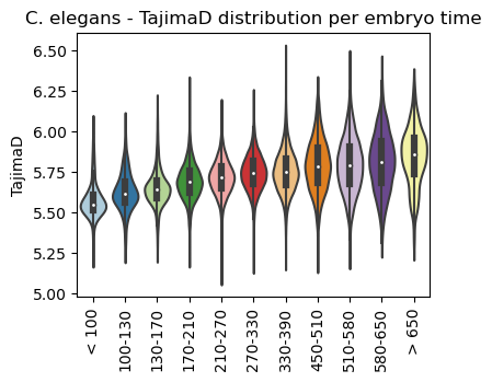
../_images/notebooks_nematode_example_46_0.png

Boxplot TajimaD class per sample timepoint

[24]:

ax = sc.pl.violin(adata=celegans_data,
                  keys=['TajimaD'],
                  groupby='embryo.time.bin.cat',
                  rotation=90,
                  palette='Paired',
                  stripplot=False,
                  inner='box',
                  order=['< 100', '100-130', '130-170', '170-210',
                         '210-270', '270-330', '330-390', '450-510',
                         '510-580', '580-650', '> 650'],
                  show=False)
ax.set_title('C. elegans - TajimaD distribution per embryo time')
plt.show()

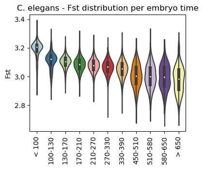
../_images/notebooks_nematode_example_48_0.png

Boxplot Fst class per sample timepoint

[25]:

ax = sc.pl.violin(adata=celegans_data,
                  keys=['Fst'],
                  groupby='embryo.time.bin.cat',
                  rotation=90,
                  palette='Paired',
                  stripplot=False,
                  inner='box',
                  order=['< 100', '100-130', '130-170', '170-210',
                         '210-270', '270-330', '330-390', '450-510',
                         '510-580', '580-650', '> 650'],
                  show=False)
ax.set_title('C. elegans - Fst distribution per embryo time')
plt.show()

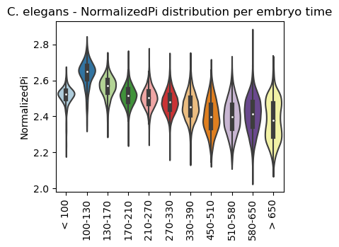
../_images/notebooks_nematode_example_50_0.png

Boxplot NormalizedPi class per sample timepoint

[26]:

ax = sc.pl.violin(adata=celegans_data,
                  keys=['NormalizedPi'],
                  groupby='embryo.time.bin.cat',
                  rotation=90,
                  palette='Paired',
                  stripplot=False,
                  inner='box',
                  order=['< 100', '100-130', '130-170', '170-210',
                         '210-270', '270-330', '330-390', '450-510',
                         '510-580', '580-650', '> 650'],
                  show=False)
ax.set_title('C. elegans - NormalizedPi distribution per embryo time')
plt.show()

../_images/notebooks_nematode_example_52_0.png

Boxplot gene age class per sample timepoint and add significance

Note: Please change notebook cell from raw to code to see the plots.

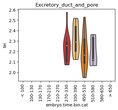
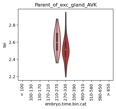
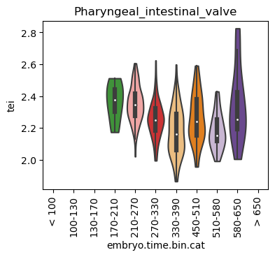
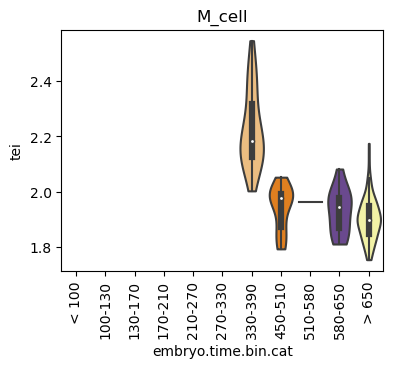
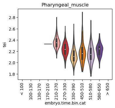
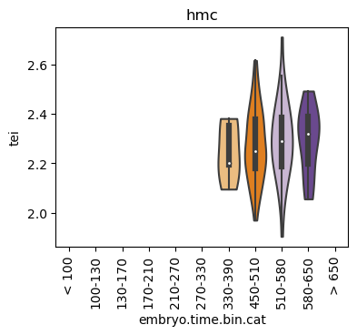
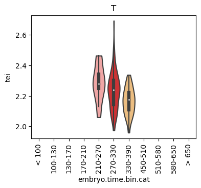
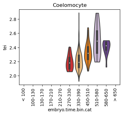
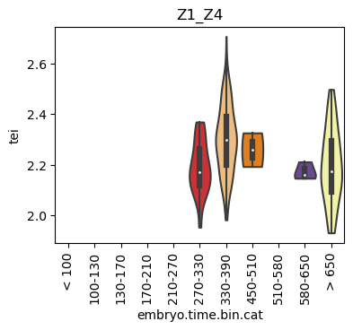
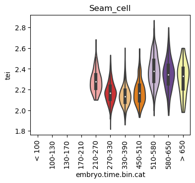
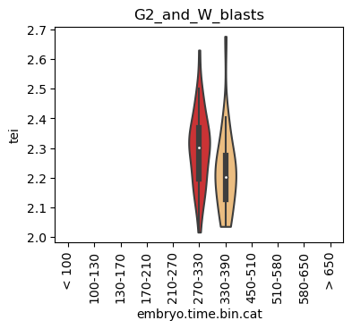
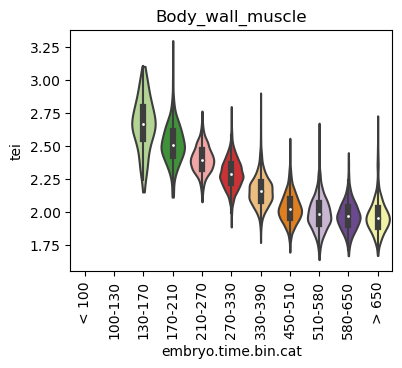
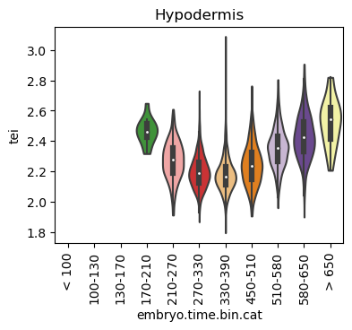
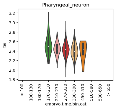
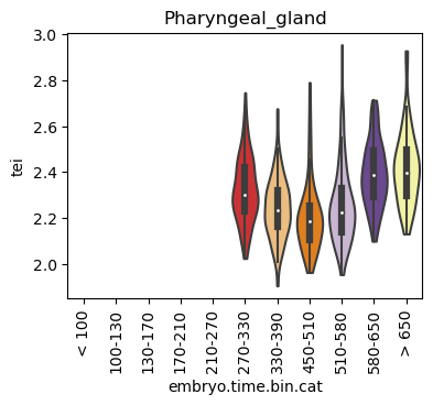
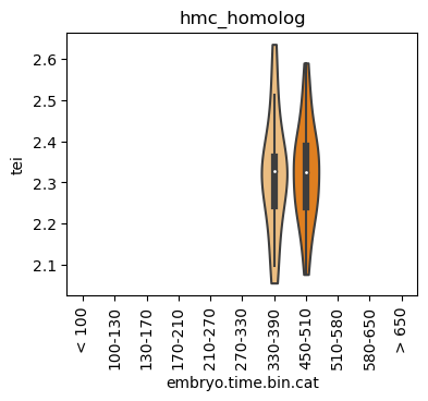
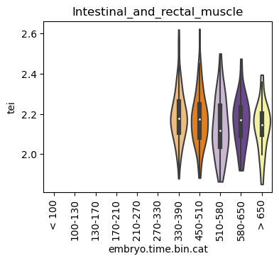
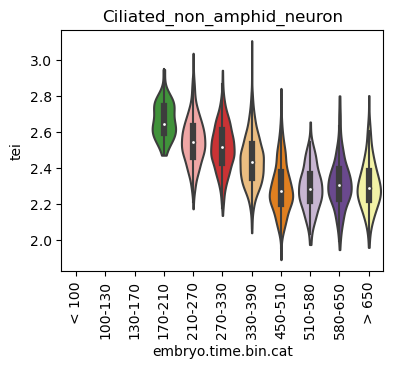
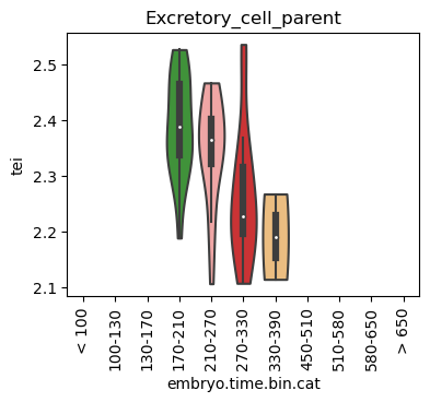
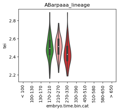
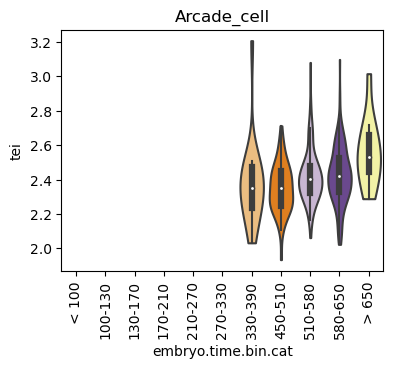
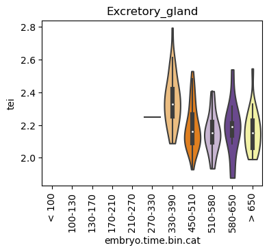
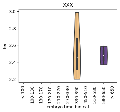
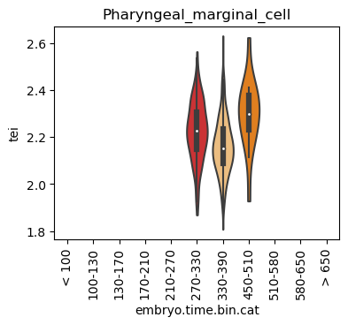
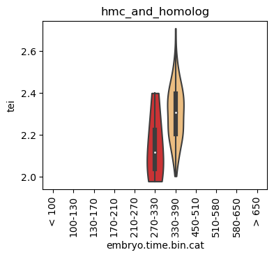
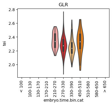
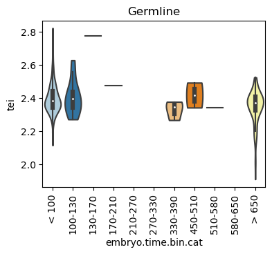
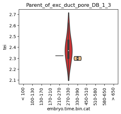
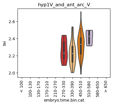
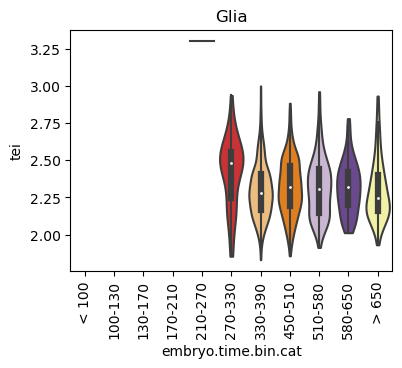
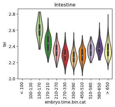
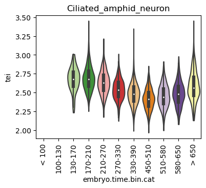
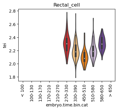
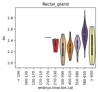
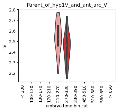
ax = sns.boxplot( x='embryo.time.bin.cat', y='tei', data=celegans_data.obs) ax.set_title('C. elegans - TEI distribution per embryo time') test_results = add_stat_annotation( ax, x='embryo.time.bin.cat', y='tei', data=celegans_data.obs, box_pairs=orthomap2tei._get_pairwise_comb_self( list1=celegans_data.obs['embryo.time.bin.cat'].value_counts().index), test='Mann-Whitney', text_format='star', loc='outside', verbose=0) plt.xticks(rotation=90) plt.show()

Boxplot gene age class per sample timepoint and per cell type

E.g. to just show the same plot for a selected cell-type, one could do the following.

List all annotated cell types:

[27]:

list(set(celegans_data.obs['cell.type']))

[27]:

['Excretory_duct_and_pore',
 'Parent_of_exc_gland_AVK',
 'Pharyngeal_intestinal_valve',
 'M_cell',
 'Pharyngeal_muscle',
 'hmc',
 'T',
 'Coelomocyte',
 'Z1_Z4',
 'Seam_cell',
 'G2_and_W_blasts',
 'Body_wall_muscle',
 'Hypodermis',
 'Pharyngeal_neuron',
 'Pharyngeal_gland',
 'hmc_homolog',
 'Intestinal_and_rectal_muscle',
 'Ciliated_non_amphid_neuron',
 'Excretory_cell_parent',
 'ABarpaaa_lineage',
 'Arcade_cell',
 'Excretory_gland',
 'XXX',
 'Pharyngeal_marginal_cell',
 'Excretory_cell',
 'hmc_and_homolog',
 'NA',
 'GLR',
 'Germline',
 'Parent_of_exc_duct_pore_DB_1_3',
 'hyp1V_and_ant_arc_V',
 'Glia',
 'Intestine',
 'Ciliated_amphid_neuron',
 'Rectal_cell',
 'Rectal_gland',
 'Parent_of_hyp1V_and_ant_arc_V']

Loop over all cell types:

Note: Please change notebook cell from raw to code to see the plots.

[28]:

for ct in list(set(celegans_data.obs['cell.type'])):
    ax = sc.pl.violin(adata=celegans_data[celegans_data.obs['cell.type']==ct],
                      keys=['tei'],
                      groupby='embryo.time.bin.cat',
                      rotation=90,
                      palette='Paired',
                      stripplot=False,
                      inner='box',
                      order=['< 100', '100-130', '130-170', '170-210',
                             '210-270', '270-330', '330-390', '450-510',
                             '510-580', '580-650', '> 650'],
                      show=False)
    ax.set_title(ct)
    ax.set_xlabel('embryo.time.bin.cat')
    plt.show()

../_images/notebooks_nematode_example_59_0.png

../_images/notebooks_nematode_example_59_1.png

../_images/notebooks_nematode_example_59_2.png

../_images/notebooks_nematode_example_59_3.png

../_images/notebooks_nematode_example_59_4.png

../_images/notebooks_nematode_example_59_5.png

../_images/notebooks_nematode_example_59_6.png

../_images/notebooks_nematode_example_59_7.png

../_images/notebooks_nematode_example_59_8.png

../_images/notebooks_nematode_example_59_9.png

../_images/notebooks_nematode_example_59_10.png

../_images/notebooks_nematode_example_59_11.png

../_images/notebooks_nematode_example_59_12.png

../_images/notebooks_nematode_example_59_13.png

../_images/notebooks_nematode_example_59_14.png

../_images/notebooks_nematode_example_59_15.png

../_images/notebooks_nematode_example_59_16.png

../_images/notebooks_nematode_example_59_17.png

../_images/notebooks_nematode_example_59_18.png

../_images/notebooks_nematode_example_59_19.png

../_images/notebooks_nematode_example_59_20.png

../_images/notebooks_nematode_example_59_21.png

../_images/notebooks_nematode_example_59_22.png

../_images/notebooks_nematode_example_59_23.png

../_images/notebooks_nematode_example_59_24.png

../_images/notebooks_nematode_example_59_25.png

../_images/notebooks_nematode_example_59_26.png

../_images/notebooks_nematode_example_59_27.png

../_images/notebooks_nematode_example_59_28.png

../_images/notebooks_nematode_example_59_29.png

../_images/notebooks_nematode_example_59_30.png

../_images/notebooks_nematode_example_59_31.png

../_images/notebooks_nematode_example_59_32.png

../_images/notebooks_nematode_example_59_33.png

../_images/notebooks_nematode_example_59_34.png

../_images/notebooks_nematode_example_59_35.png

../_images/notebooks_nematode_example_59_36.png

Scatterplot TEI vs TajimaD and color each cell by sample timepoint per cell type

Note: Please change notebook cell from raw to code to see the plots.

for ct in list(set(celegans_data.obs['cell.type'])): ax = sns.scatterplot(data=celegans_data[celegans_data.obs['cell.type']==ct].obs, x='TajimaD', y='tei', hue='embryo.time.bin.cat') ax.set_title(ct) sns.move_legend(ax, 'upper left', bbox_to_anchor=(1, 1)) plt.show()

Scatterplot TEI vs Fst and color each cell by sample timepoint per cell type

Note: Please change notebook cell from raw to code to see the plots.

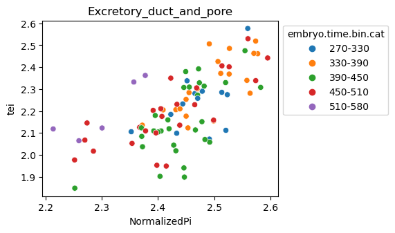
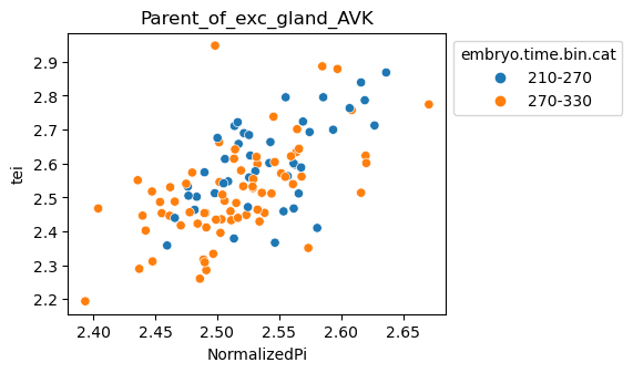
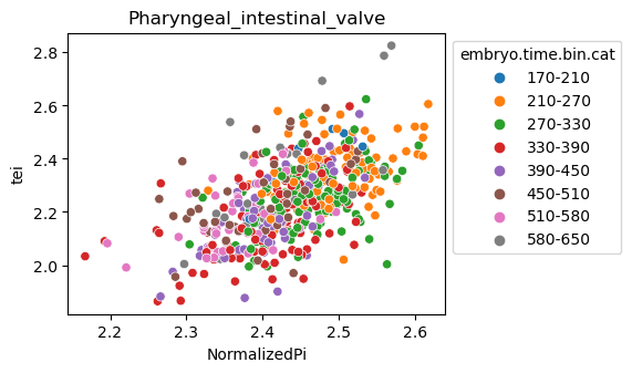
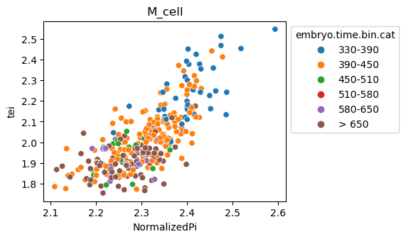
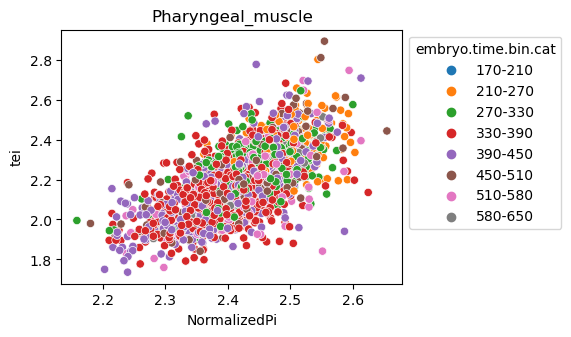
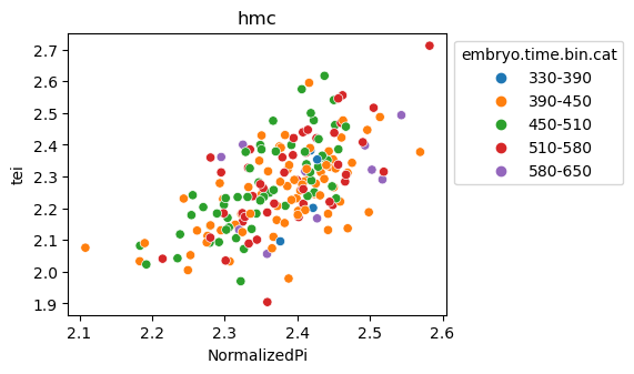
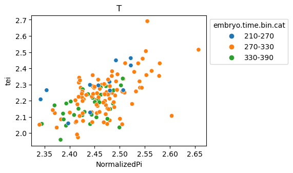
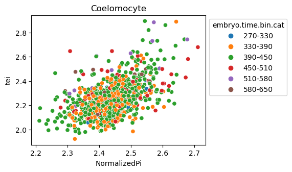
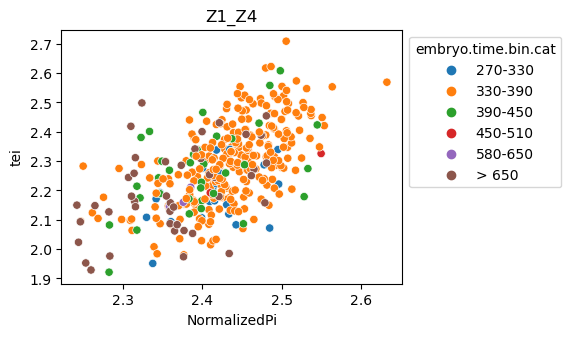
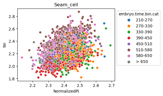
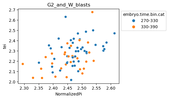
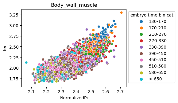
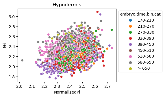
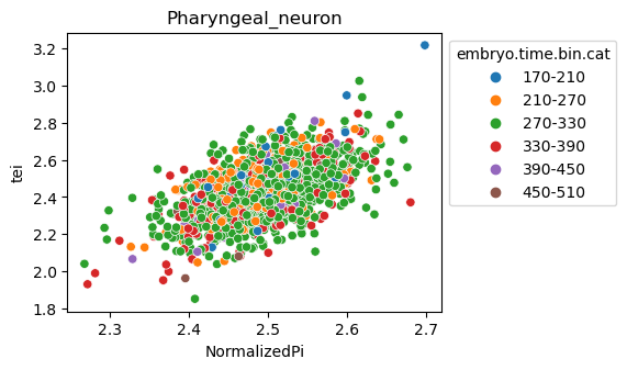
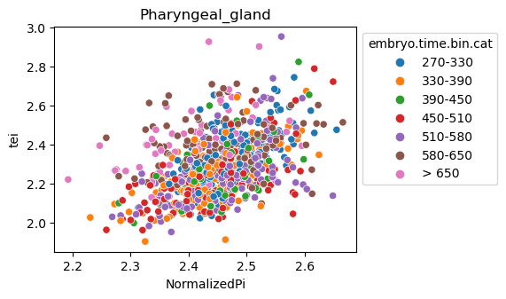
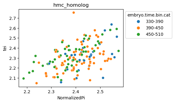
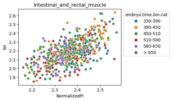
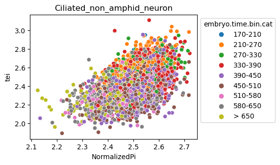
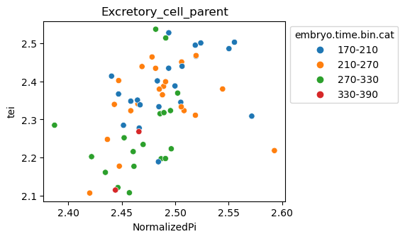
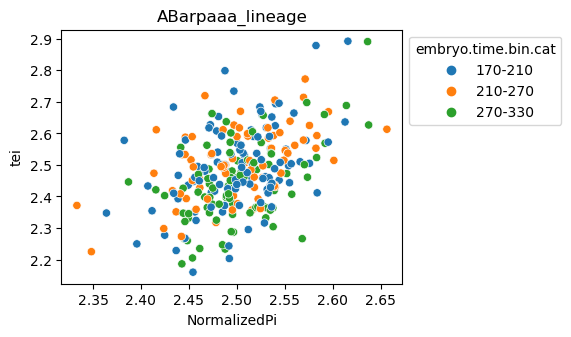
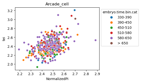
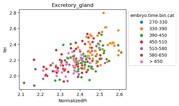
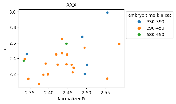
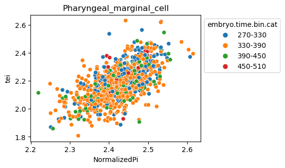
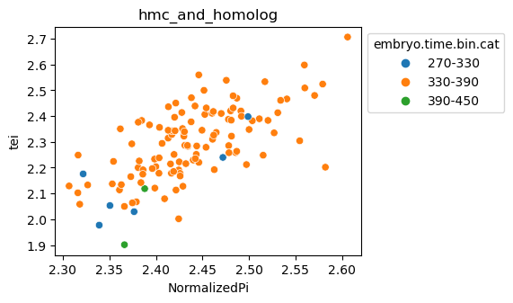
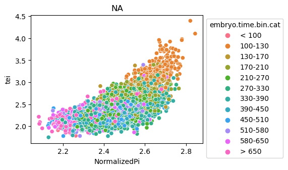
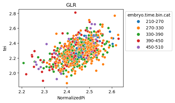
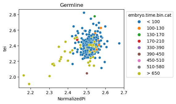
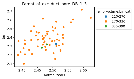
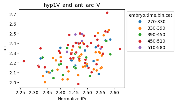
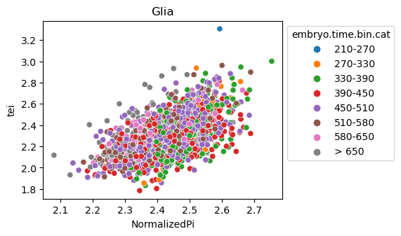
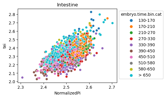
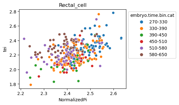
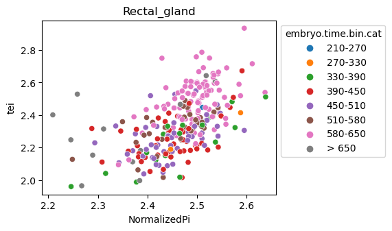
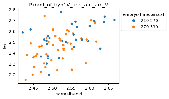
for ct in list(set(celegans_data.obs['cell.type'])): ax = sns.scatterplot(data=celegans_data[celegans_data.obs['cell.type']==ct].obs, x='Fst', y='tei', hue='embryo.time.bin.cat') ax.set_title(ct) sns.move_legend(ax, 'upper left', bbox_to_anchor=(1, 1)) plt.show()

Scatterplot TEI vs NormalizedPi and color each cell by sample timepoint per cell type

Note: Please change notebook cell from raw to code to see the plots.

[29]:

for ct in list(set(celegans_data.obs['cell.type'])):
    ax = sns.scatterplot(data=celegans_data[celegans_data.obs['cell.type']==ct].obs,
            x='NormalizedPi',
            y='tei',
            hue='embryo.time.bin.cat')
    ax.set_title(ct)
    sns.move_legend(ax, 'upper left', bbox_to_anchor=(1, 1))
    plt.show()

../_images/notebooks_nematode_example_65_0.png

../_images/notebooks_nematode_example_65_1.png

../_images/notebooks_nematode_example_65_2.png

../_images/notebooks_nematode_example_65_3.png

../_images/notebooks_nematode_example_65_4.png

../_images/notebooks_nematode_example_65_5.png

../_images/notebooks_nematode_example_65_6.png

../_images/notebooks_nematode_example_65_7.png

../_images/notebooks_nematode_example_65_8.png

../_images/notebooks_nematode_example_65_9.png

../_images/notebooks_nematode_example_65_10.png

../_images/notebooks_nematode_example_65_11.png

../_images/notebooks_nematode_example_65_12.png

../_images/notebooks_nematode_example_65_13.png

../_images/notebooks_nematode_example_65_14.png

../_images/notebooks_nematode_example_65_15.png

../_images/notebooks_nematode_example_65_16.png

../_images/notebooks_nematode_example_65_17.png

../_images/notebooks_nematode_example_65_18.png

../_images/notebooks_nematode_example_65_19.png

../_images/notebooks_nematode_example_65_20.png

../_images/notebooks_nematode_example_65_21.png

../_images/notebooks_nematode_example_65_22.png

../_images/notebooks_nematode_example_65_23.png

../_images/notebooks_nematode_example_65_24.png

../_images/notebooks_nematode_example_65_25.png

../_images/notebooks_nematode_example_65_26.png

../_images/notebooks_nematode_example_65_27.png

../_images/notebooks_nematode_example_65_28.png

../_images/notebooks_nematode_example_65_29.png

../_images/notebooks_nematode_example_65_30.png

../_images/notebooks_nematode_example_65_31.png

../_images/notebooks_nematode_example_65_32.png

../_images/notebooks_nematode_example_65_33.png

../_images/notebooks_nematode_example_65_34.png

../_images/notebooks_nematode_example_65_35.png

../_images/notebooks_nematode_example_65_36.png

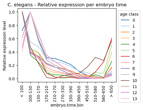
Plot relative expression per gene age class per sample timepoint

[30]:

celegans_data_rematrix_grouped = orthomap2tei.get_rematrix(
    adata=celegans_data,
    gene_id=query_orthomap['GeneID'],
    gene_age=query_orthomap['Phylostratum'],
    keep='min',
    layer=None,
    use='counts',
    var_type='mean',
    group_by_obs='embryo.time.bin.cat',
    obs_fillna='__NaN',
    obs_type='mean',
    standard_scale=0,
    normalize_total=True,
    log1p=True,
    target_sum=1e6)
celegans_data_rematrix_grouped

[30]:

embryo.time.bin.cat	< 100	100-130	130-170	170-210	210-270	270-330	330-390	390-450	450-510	510-580	580-650	> 650
ps
0	0.717118	1.000000	0.584168	0.310426	0.302204	0.260612	0.206768	0.105727	0.048908	0.000000	0.013732	0.073366
1	1.000000	0.547242	0.477675	0.295885	0.250502	0.231566	0.176154	0.112925	0.089850	0.033621	0.000000	0.165599
2	1.000000	0.450475	0.387854	0.213375	0.168202	0.154225	0.113436	0.062726	0.048594	0.026063	0.000000	0.171621
3	1.000000	0.456666	0.312041	0.126569	0.089371	0.076377	0.078763	0.018744	0.046053	0.002353	0.000000	0.394810
4	1.000000	0.351679	0.245304	0.080961	0.056258	0.050955	0.028812	0.000000	0.017548	0.057651	0.015902	0.256118
5	1.000000	0.454323	0.381592	0.113054	0.024290	0.000000	0.019198	0.011902	0.006195	0.088254	0.077768	0.503433
6	1.000000	0.393570	0.331241	0.082090	0.019724	0.015556	0.019509	0.000000	0.010253	0.100935	0.250751	0.605489
7	1.000000	0.404537	0.296849	0.164328	0.114308	0.089470	0.035970	0.005399	0.000000	0.015025	0.024354	0.153953
8	1.000000	0.374614	0.332113	0.229286	0.175440	0.116940	0.052691	0.001487	0.004222	0.003206	0.000000	0.105183
9	1.000000	0.421409	0.314549	0.205528	0.172487	0.141735	0.098434	0.040396	0.017756	0.011292	0.000000	0.105804
10	1.000000	0.473084	0.224513	0.014137	0.000000	0.042069	0.067210	0.077679	0.173604	0.316754	0.270774	0.566895
11	0.613516	1.000000	0.562404	0.273833	0.202082	0.145245	0.092380	0.043486	0.033280	0.000000	0.003208	0.043322
12	0.470709	1.000000	0.665627	0.351440	0.257487	0.176988	0.101492	0.025500	0.011935	0.000000	0.000159	0.055289
13	0.411756	1.000000	0.649935	0.344974	0.252738	0.172185	0.096022	0.034795	0.025026	0.004728	0.000000	0.057878

[31]:

ax = sns.lineplot(celegans_data_rematrix_grouped.transpose(), palette='tab20', dashes=False)
ax.legend(fontsize=5, title='age class')
ax.set_title('C. elegans - Relative expression per embryo time')
ax.set_xlabel('embryo.time.bin')
ax.set_ylabel('Relative expression level')
sns.move_legend(ax, 'upper left', bbox_to_anchor=(1, 1))
plt.xticks(rotation=90)
plt.show()

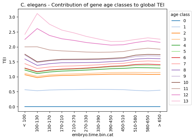
../_images/notebooks_nematode_example_68_0.png

Get partial TEI values to visualize gene age class contributions

Partial TEI values can give an idea about which gene age class contributed at most to the global TEI pattern.

In detail, each gene gets a TEI contribution profile as follows:

\({TEI_{is} = f_{is} * ps_i}\)

, where \({TEI_{is}}\) is the partial TEI value of gene \({i}\), \({f_{is} = e_{is} / \sum e_{is}}\) and \({ps_i}\) is the phylostratum of gene i.

\({TEI_{is}}\) values are combined per \({ps}\).

The partial TEI values combined per strata give an overall impression of the contribution of each strata to the global TEI pattern.

One can either start from counts (adata.X) which is set as default or any other layer defined by the layer option (layer=None).

In addition, the counts can be normalized and log-transformed prior calculating partial TEI values (normalize_total=False, log1p=False, target_sum=1e6).

Further, these values can be combined per given observation, e.g. sample timepoint (group_by='raw.embryo.time').

The get_pstrata function of the orthomap2tei submodule will return two matrix, the first contains the sum of each partial TEI per gene age class and the second the corresponding frequencies.

Both can be further processed by returning the cumsum over the gene age classes. To get them set the option cumsum=True. The cumsum will result in either for the first matrix the TEI value per cell or mean TEI value per group, if one choose a observation with the group_by option. Or in case of the second frequency matrix will result in 1.

With the standard_scale option either gene age classes (standard_scale=0 rows) or cells or groups (standard_scale=1 columns) can be scaled, subtract the minimum and divide each by its maximum. By default no scaling is applied (standard_scale=None).

The resulting data will be visualized in the downstream section.

[32]:

celegans_pstrata = orthomap2tei.get_pstrata(adata=celegans_data,
    gene_id=query_orthomap['GeneID'],
    gene_age=query_orthomap['Phylostratum'],
    keep='min',
    layer=None,
    cumsum=True,
    group_by_obs='embryo.time.bin.cat',
    obs_fillna='__NaN',
    obs_type='mean',
    standard_scale=None,
    normalize_total=True,
    log1p=True,
    target_sum=1e6)
celegans_pstrata[0]

[32]:

embryo.time.bin.cat	< 100	100-130	130-170	170-210	210-270	270-330	330-390	390-450	450-510	510-580	580-650	> 650
ps
0	0.000000	0.000000	0.000000	0.000000	0.000000	0.000000	0.000000	0.000000	0.000000	0.000000	0.000000	0.000000
1	0.564379	0.530493	0.554769	0.564274	0.568691	0.574967	0.574761	0.572603	0.567071	0.540339	0.525781	0.547670
2	1.066948	0.969366	1.019430	1.040665	1.048817	1.063191	1.072649	1.085847	1.086674	1.085105	1.076311	1.078825
3	1.110209	1.010589	1.060572	1.084848	1.094679	1.110265	1.124388	1.139774	1.144051	1.145294	1.139959	1.142614
4	1.222601	1.106044	1.157717	1.187257	1.202083	1.221465	1.242487	1.266474	1.278308	1.303513	1.299550	1.289389
5	1.269068	1.150924	1.206516	1.236391	1.250166	1.269788	1.296496	1.326829	1.340107	1.379603	1.379764	1.367366
6	1.288148	1.168326	1.225392	1.255229	1.269197	1.289450	1.318017	1.350846	1.364751	1.410713	1.419942	1.404574
7	1.436406	1.275586	1.325999	1.352471	1.361118	1.378901	1.398513	1.431710	1.446642	1.507610	1.527176	1.513817
8	1.593160	1.379820	1.436263	1.467291	1.469098	1.473799	1.480398	1.503826	1.523043	1.589848	1.613239	1.603044
9	1.723074	1.475801	1.529523	1.564003	1.566499	1.568462	1.572929	1.588345	1.603053	1.674875	1.700259	1.690460
10	1.750491	1.499340	1.549016	1.580853	1.584175	1.588804	1.596092	1.614562	1.635971	1.721640	1.746472	1.738911
11	1.998728	2.001177	1.895514	1.864111	1.846383	1.824879	1.817629	1.822785	1.842534	1.912595	1.954244	1.922988
12	2.249283	2.611671	2.381169	2.269536	2.214056	2.144069	2.100194	2.057414	2.069561	2.143782	2.200446	2.149454
13	2.419276	3.114069	2.756838	2.561030	2.465832	2.348615	2.261164	2.178997	2.185036	2.246225	2.300599	2.255455

corresponds to main figure Figure 1E

[33]:

plt.rcParams['figure.figsize'] = [6.5, 4.5]
ax = sns.lineplot(celegans_pstrata[0].transpose(), palette='tab20', dashes=False)
ax.legend(fontsize=3, title='age class')
ax.set_title('C. elegans - Contribution of gene age classes to global TEI')
ax.set_xlabel('embryo.time.bin.cat')
ax.set_ylabel('TEI')
sns.move_legend(ax, 'upper left', bbox_to_anchor=(1, 1))
plt.xticks(rotation=90)
plt.show()
plt.rcParams['figure.figsize'] = [4.4, 3.3]

../_images/notebooks_nematode_example_72_0.png

partial TajimaD

Note: Please change notebook cell from raw to code to see the plots.

celegans_pstrata_tajimaD = orthomap2tei.get_pstrata(adata=celegans_data, gene_id=query_fst['WormBase_ID'], gene_age=query_fst['TajimaD_binned'], keep='min', layer=None, cumsum=False, group_by_obs='raw.embryo.time', obs_fillna='__NaN', obs_type='mean', standard_scale=None, normalize_total=True, log1p=True, target_sum=1e6) celegans_pstrata_tajimaD[0]

Note: Please change notebook cell from raw to code to see the plots.

ax=celegans_pstrata_tajimaD[0].transpose().plot.area(cmap='tab20') ax.legend(fontsize=3, title='age class') ax.set_title('C. elegans - Contribution of TajimaD classes to global TajimaD') ax.set_xlabel('raw.embryo.time') ax.set_ylabel('TajimaD') sns.move_legend(ax, 'upper left', bbox_to_anchor=(1, 1)) plt.xticks(rotation=90) plt.show()

partial Fst

Note: Please change notebook cell from raw to code to see the plots.

celegans_pstrata_Fst = orthomap2tei.get_pstrata(adata=celegans_data, gene_id=query_fst['WormBase_ID'], gene_age=query_fst['FST_binned'], keep='min', layer=None, cumsum=False, group_by_obs='raw.embryo.time', obs_fillna='__NaN', obs_type='mean', standard_scale=None, normalize_total=True, log1p=True, target_sum=1e6) celegans_pstrata_Fst[0]

Note: Please change notebook cell from raw to code to see the plots.

ax=celegans_pstrata_Fst[0].transpose().plot.area(cmap='tab20') ax.legend(fontsize=3, title='age class') ax.set_title('C. elegans - Contribution of Fst classes to global Fst') ax.set_xlabel('raw.embryo.time') ax.set_ylabel('Fst') sns.move_legend(ax, 'upper left', bbox_to_anchor=(1, 1)) plt.xticks(rotation=90) plt.show()

partial NormalizedPi

Note: Please change notebook cell from raw to code to see the plots.

celegans_pstrata_normPi = orthomap2tei.get_pstrata(adata=celegans_data, gene_id=query_fst['WormBase_ID'], gene_age=query_fst['NormalizedPi_binned'], keep='min', layer=None, cumsum=False, group_by_obs='raw.embryo.time', obs_fillna='__NaN', obs_type='mean', standard_scale=None, normalize_total=True, log1p=True, target_sum=1e6) celegans_pstrata_normPi[0]

Note: Please change notebook cell from raw to code to see the plots.

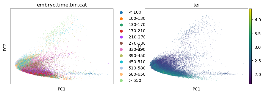
ax=celegans_pstrata_normPi[0].transpose().plot.area(cmap='tab20') ax.legend(fontsize=3, title='age class') ax.set_title('C. elegans - Contribution of NormalizedPi classes to global NormalizedPi') ax.set_xlabel('raw.embryo.time') ax.set_ylabel('NormalizedPi') sns.move_legend(ax, 'upper left', bbox_to_anchor=(1, 1)) plt.xticks(rotation=90) plt.show()

Color UMAP/TSNE by TEI

Follwoing the basic tutorial of the Scanpy python toolkit (Wolf et al., 2018), one can highlight TEI values on a dimensional reduction of the scRNA dataset, like PCA, UMAP or TSNE.

Filtering

[34]:

sc.pp.filter_genes(celegans_data, min_cells=3)
sc.pp.filter_cells(celegans_data, min_genes=200)

Normalization, Log transformation and Scaling

[35]:

sc.pp.normalize_total(celegans_data, target_sum=1e6)
sc.pp.log1p(celegans_data)
sc.pp.scale(celegans_data, max_value=10)

PCA and Neighbor calculations

[36]:

sc.tl.pca(celegans_data, svd_solver='arpack')
sc.pl.pca(celegans_data, color=['embryo.time.bin.cat', 'tei'])

/opt/anaconda3/envs/scanpy/lib/python3.8/site-packages/scanpy/plotting/_tools/scatterplots.py:392: UserWarning: No data for colormapping provided via 'c'. Parameters 'cmap' will be ignored
  cax = scatter(

../_images/notebooks_nematode_example_91_1.png

[37]:

sc.pp.neighbors(celegans_data)

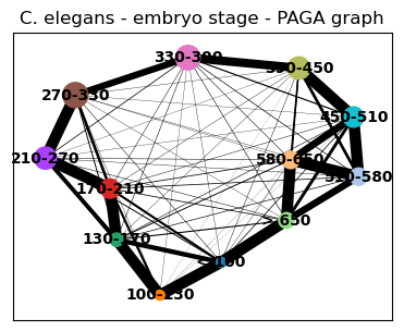
Embedding the neighborhood graph

[38]:

sc.tl.paga(celegans_data, groups='embryo.time.bin.cat')
sc.pl.paga(celegans_data, title='C. elegans - embryo stage - PAGA graph')

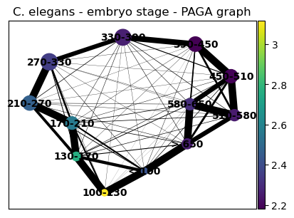
../_images/notebooks_nematode_example_94_0.png

[39]:

sc.pl.paga(celegans_data, title='C. elegans - embryo stage - PAGA graph', color=['tei'])

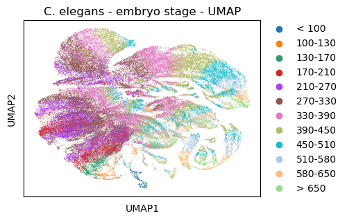
../_images/notebooks_nematode_example_95_0.png

UMAP

[40]:

sc.tl.umap(celegans_data,
           init_pos='paga')
sc.pl.umap(celegans_data,
           title='C. elegans - embryo stage - UMAP', color=['embryo.time.bin.cat'])

/opt/anaconda3/envs/scanpy/lib/python3.8/site-packages/scanpy/plotting/_tools/scatterplots.py:392: UserWarning: No data for colormapping provided via 'c'. Parameters 'cmap' will be ignored
  cax = scatter(

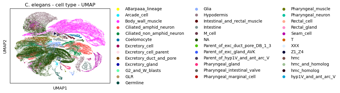
../_images/notebooks_nematode_example_97_1.png

Color UMAP by cell type

[41]:

sc.pl.umap(celegans_data,
           title='C. elegans - cell type - UMAP', color=['cell.type'])

/opt/anaconda3/envs/scanpy/lib/python3.8/site-packages/scanpy/plotting/_tools/scatterplots.py:392: UserWarning: No data for colormapping provided via 'c'. Parameters 'cmap' will be ignored
  cax = scatter(

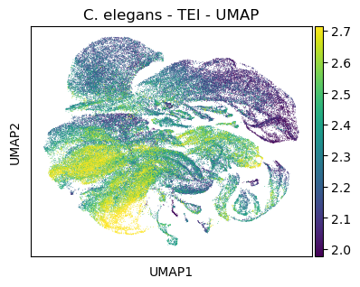
../_images/notebooks_nematode_example_99_1.png

Color UMAP by TEI

[42]:

#plt.rcParams['figure.figsize'] = [7.5, 4.5]
sc.pl.umap(celegans_data,
           title='C. elegans - TEI - UMAP',
           color=['tei'],
           color_map='viridis',
           vmin='p5',
           vmax='p95')
#plt.rcParams['figure.figsize'] = [6, 4.5]

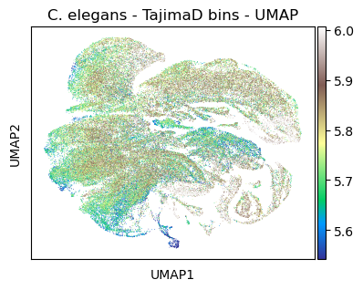
../_images/notebooks_nematode_example_101_0.png

Color UMAP by TajimaD bins

[43]:

#plt.rcParams['figure.figsize'] = [7.5, 4.5]
sc.pl.umap(celegans_data,
           title='C. elegans - TajimaD bins - UMAP',
           color=['TajimaD'],
           color_map='terrain',
           vmin='p5',
           vmax='p95')
#plt.rcParams['figure.figsize'] = [6, 4.5]

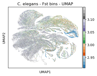
../_images/notebooks_nematode_example_103_0.png

Color UMAP by Fst bins

[44]:

#plt.rcParams['figure.figsize'] = [7.5, 4.5]
sc.pl.umap(celegans_data,
           title='C. elegans - Fst bins - UMAP',
           color=['Fst'],
           color_map='tab20c',
           vmin='p5',
           vmax='p95')
#plt.rcParams['figure.figsize'] = [6, 4.5]

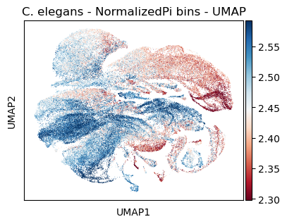
../_images/notebooks_nematode_example_105_0.png

Color UMAP by NormalizedPi bins

[45]:

#plt.rcParams['figure.figsize'] = [7.5, 4.5]
sc.pl.umap(celegans_data,
           title='C. elegans - NormalizedPi bins - UMAP',
           color=['NormalizedPi'],
           color_map='RdBu',
           vmin='p5',
           vmax='p95')
#plt.rcParams['figure.figsize'] = [6, 4.5]

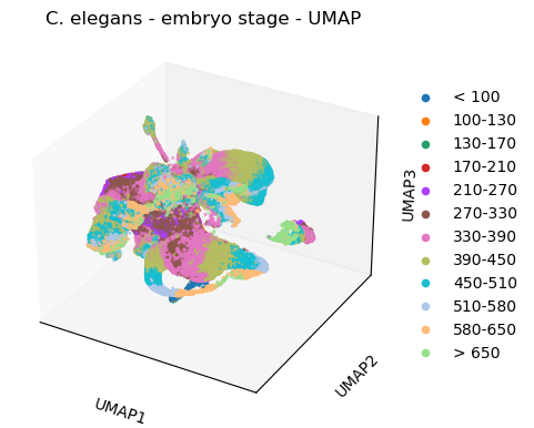
../_images/notebooks_nematode_example_107_0.png

3D-UMAP

[46]:

plt.rcParams['figure.figsize'] = [7.5, 4.5]
#3d
sc.tl.umap(celegans_data,
           n_components=3)
sc.pl.umap(celegans_data,
           title='C. elegans - embryo stage - UMAP',
           color=['embryo.time.bin.cat'],
           projection='3d')
plt.rcParams['figure.figsize'] = [4.4, 3.3]

/opt/anaconda3/envs/scanpy/lib/python3.8/site-packages/scanpy/plotting/_tools/scatterplots.py:325: UserWarning: No data for colormapping provided via 'c'. Parameters 'cmap' will be ignored
  cax = ax.scatter(

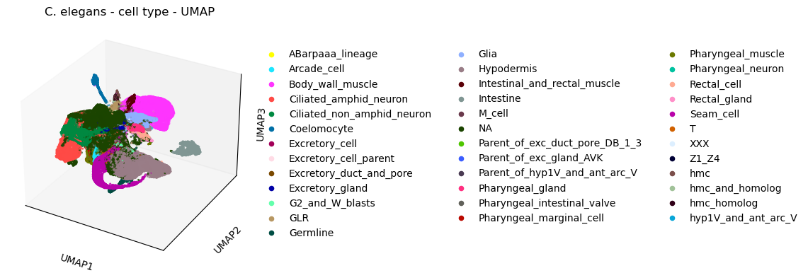
../_images/notebooks_nematode_example_109_1.png

[47]:

plt.rcParams['figure.figsize'] = [7.5, 4.5]
#3d
sc.pl.umap(celegans_data,
           title='C. elegans - cell type - UMAP',
           color=['cell.type'],
           projection='3d')
plt.rcParams['figure.figsize'] = [4.4, 3.3]

/opt/anaconda3/envs/scanpy/lib/python3.8/site-packages/scanpy/plotting/_tools/scatterplots.py:325: UserWarning: No data for colormapping provided via 'c'. Parameters 'cmap' will be ignored
  cax = ax.scatter(

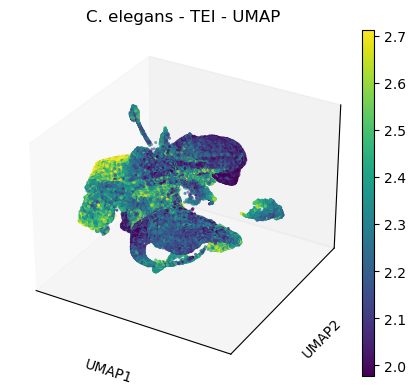
../_images/notebooks_nematode_example_110_1.png

[48]:

plt.rcParams['figure.figsize'] = [7.5, 4.5]
#3d
sc.pl.umap(celegans_data,
           title='C. elegans - TEI - UMAP',
           color=['tei'],
           color_map='viridis',
           vmin='p5',
           vmax='p95',
           projection='3d')
plt.rcParams['figure.figsize'] = [4.4, 3.3]

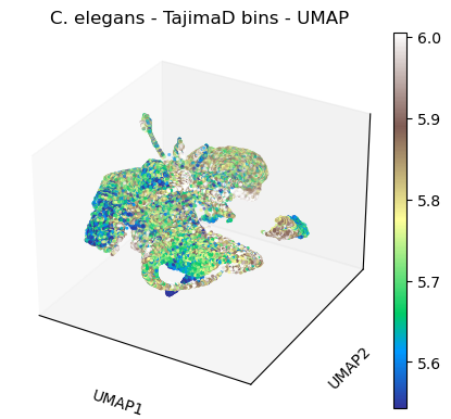
../_images/notebooks_nematode_example_111_0.png

[49]:

plt.rcParams['figure.figsize'] = [7.5, 4.5]
#3d
sc.pl.umap(celegans_data,
           title='C. elegans - TajimaD bins - UMAP',
           color=['TajimaD'],
           color_map='terrain',
           vmin='p5',
           vmax='p95',
           projection='3d')
plt.rcParams['figure.figsize'] = [4.4, 3.3]

../_images/notebooks_nematode_example_112_0.png

[50]:

plt.rcParams['figure.figsize'] = [7.5, 4.5]
sc.pl.umap(celegans_data,
           title='C. elegans - Fst bins - UMAP',
           color=['Fst'],
           color_map='tab20c',
           vmin='p5',
           vmax='p95',
           projection='3d')
plt.rcParams['figure.figsize'] = [4.4, 3.3]

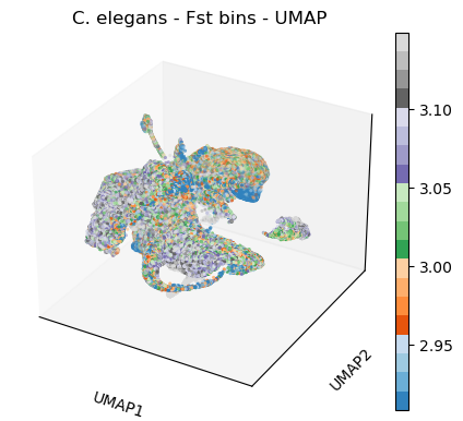
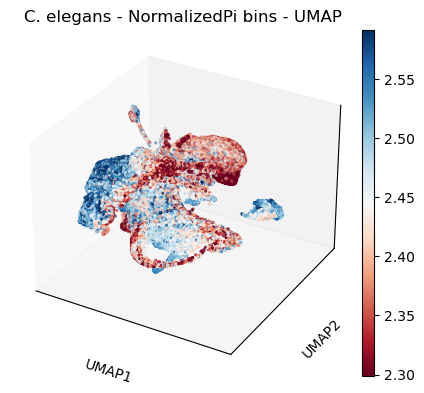
../_images/notebooks_nematode_example_113_0.png

[51]:

plt.rcParams['figure.figsize'] = [7.5, 4.5]
#3d
sc.pl.umap(celegans_data,
           title='C. elegans - NormalizedPi bins - UMAP',
           color=['NormalizedPi'],
           color_map='RdBu',
           vmin='p5',
           vmax='p95',
           projection='3d')
plt.rcParams['figure.figsize'] = [4.4, 3.3]

../_images/notebooks_nematode_example_114_0.png

Please have a look at the documentation for other case studies.