Case study: re-analysis myeloid and erythroid differentiation of mouse (Mus musculus) single-cell data
This notebook will demonstrate scRNA-seq processing with oggmap using mouse scRNA data from Paul et al., 2015.
scRNA data was obtained via Scanpy (Wolf et al., 2018).
see also:
Notebook file
Notebook file can be obtained here:
https://raw.githubusercontent.com/kullrich/oggmap/main/docs/notebooks/paul15_example.ipynb
Steps
To process the scRNA data, we will do the following:
Run OrthoFinder to obtain orthogroups
Get query species taxonomic lineage information
Get query species orthomap
Map OrthoFinder gene names and scRNA gene/transcript names
Get TEI values and add them to scRNA dataset
Get partial TEI values to visualize gene age class contributions
Process scRNA data and visualize TEI
Import libraries
[1]:
import numpy as np
import pandas as pd
import scanpy as sc
import seaborn as sns
import matplotlib.pyplot as plt
from statannot import add_stat_annotation
# increase dpi
%matplotlib inline
#plt.rcParams['figure.dpi'] = 300
#plt.rcParams['savefig.dpi'] = 300
plt.rcParams['figure.figsize'] = [6, 4.5]
#plt.rcParams['figure.figsize'] = [4.4, 3.3]
Import oggmap python package submodules
[2]:
# import submodules
from oggmap import qlin, gtf2t2g, of2orthomap, orthomap2tei, datasets
Step 0 - run OrthoFinder to obtain orthogroups
oggmap can extract gene age classification from existing OrthoFinder results and link them with scRNA data.
A detailed how-to is available here:
https://oggmap.readthedocs.io/en/latest/tutorials/orthofinder.html
However, any pre-calculated gene age classification can be imported as a table using the function orthomap2tei.read_orthomap(orthomapfile=filename).
The pre-calculated gene age classification file should be delimited with two columns GeneID<tab>Phylostratum, like e.g.:
GeneID<tab>Phylostratum
WBGene00000001<tab>1
WBGene00000002<tab>1
WBGene00000003<tab>1
WBGene00000004<tab>1
WBGene00000005<tab>2
OrthoFinder (Emms and Kelly, 2019) results (-S last) using translated, longest-isoform coding sequences (CDS) from Ensembl release-110, including species taxonomic IDs, are available here:
https://doi.org/10.5281/zenodo.7242264
or can be accessed with the dataset submodule of oggmap
datasets.ensembl110_last(datapath='data') (download folder set to 'data').
To be able to process the scRNA data from Briggs et al. 2018 the OrthoFinder run for Ensembl release-110 was supplemented with the gene models of X. tropicalis v9.0 https://ftp.xenbase.org/pub/Genomics/JGI/Xentr9.0/Xtropicalisv9.0.Named.primaryTrs.pep.fa.gz.
This use case show that with OrthoFinder it is possible to add any new annotation as a new entry and use it with oggmap to extract the correspoding gene age assignments.
[3]:
datasets.ensembl110_last(datapath='data')
100% [..........................................................] 11317 / 11317
[3]:
['data/ensembl_110_orthofinder_last_Orthogroups.GeneCount.tsv.zip',
 'data/ensembl_110_orthofinder_last_Orthogroups.tsv.zip',
 'data/ensembl_110_orthofinder_last_species_list.tsv']
Step 1 - get query species taxonomic lineage information
Given a species name or taxonomic ID, the query species lineage information is extracted with the help of the ete3 python toolkit and the NCBI taxonomy (Huerta-Cepas et al., 2016). This information is needed alongside with the taxonomic classifications for all species used in the OrthoFinder comparison.
The oggmap submodule qlin helps to get this information for you with the qlin.get_qlin() function as follows:
[4]:
# get query species taxonomic lineage information
query_lineage = qlin.get_qlin(q='Mus musculus')
query name: Mus musculus
query taxID: 10090
query kingdom: Eukaryota
query lineage names:
['root(1)', 'cellular organisms(131567)', 'Eukaryota(2759)', 'Opisthokonta(33154)', 'Metazoa(33208)', 'Eumetazoa(6072)', 'Bilateria(33213)', 'Deuterostomia(33511)', 'Chordata(7711)', 'Craniata(89593)', 'Vertebrata(7742)', 'Gnathostomata(7776)', 'Teleostomi(117570)', 'Euteleostomi(117571)', 'Sarcopterygii(8287)', 'Dipnotetrapodomorpha(1338369)', 'Tetrapoda(32523)', 'Amniota(32524)', 'Mammalia(40674)', 'Theria(32525)', 'Eutheria(9347)', 'Boreoeutheria(1437010)', 'Euarchontoglires(314146)', 'Glires(314147)', 'Rodentia(9989)', 'Myomorpha(1963758)', 'Muroidea(337687)', 'Muridae(10066)', 'Murinae(39107)', 'Mus(10088)', 'Mus(862507)', 'Mus musculus(10090)']
query lineage:
[1, 131567, 2759, 33154, 33208, 6072, 33213, 33511, 7711, 89593, 7742, 7776, 117570, 117571, 8287, 1338369, 32523, 32524, 40674, 32525, 9347, 1437010, 314146, 314147, 9989, 1963758, 337687, 10066, 39107, 10088, 862507, 10090]
Step 2 - gene age class assignment (query species orthomap)
Here, oggmap use the query species information and OrthoFinder results to extract the oldest common tree node per orthogroup along a species tree and to assign this node as the gene age to the corresponding genes.
In a pairwise manner, the query species and any other species in the OrthoFinder result might share multiple tree nodes down to the root of the species tree, but have only one youngest tree node in common. Among all possible comparison between the query species and the other species, the oldest as defined by the species tree root is seected and used for the gene age assignment.
Given the query species sequence name (seqname=) used in the OrthoFinder comparison, the query species taxonomic ID(qt=), the taxonomic IDs of all species (sl=) used in the OrthoFinder comparison, the orthogroup gene count (oc=) results and the orthogroups (og=), an orthomap is constructed.
Note: This step can take up to five minutes, depending on your hardware.
For this step to get the query species orthomap, one uses the of2orthomap.get_orthomap() function, like:
[5]:
# get query species orthomap

# download orthofinder results here: https://doi.org/10.5281/zenodo.7242264
# or download with datasets.ensembl105(datapath='data')
query_orthomap, orthofinder_species_list, of_species_abundance = of2orthomap.get_orthomap(
    seqname='10090.mus_musculus.pep',
    qt='10090',
    sl='data/ensembl_110_orthofinder_last_species_list.tsv',
    oc='data/ensembl_110_orthofinder_last_Orthogroups.GeneCount.tsv.zip',
    og='data/ensembl_110_orthofinder_last_Orthogroups.tsv.zip',
    continuity=True)
query_orthomap
10090.mus_musculus.pep
Mus musculus
10090
                                    species  taxID  \
0                 10020.dipodomys_ordii.pep  10020
1    10029.cricetulus_griseus_chok1gshd.pep  10029
2       10029.cricetulus_griseus_crigri.pep  10029
3         10029.cricetulus_griseus_picr.pep  10029
4            10036.mesocricetus_auratus.pep  10036
..                                      ...    ...
313          9986.oryctolagus_cuniculus.pep   9986
314        99883.tetraodon_nigroviridis.pep  99883
315        9994.marmota_marmota_marmota.pep   9994
316            9999.urocitellus_parryii.pep   9999
317    Xtropicalisv9.0.Named.primaryTrs.pep   8364

                                               lineage  youngest_common  \
0    [1, 131567, 2759, 33154, 33208, 6072, 33213, 3...             9989
1    [1, 131567, 2759, 33154, 33208, 6072, 33213, 3...           337687
2    [1, 131567, 2759, 33154, 33208, 6072, 33213, 3...           337687
3    [1, 131567, 2759, 33154, 33208, 6072, 33213, 3...           337687
4    [1, 131567, 2759, 33154, 33208, 6072, 33213, 3...           337687
..                                                 ...              ...
313  [1, 131567, 2759, 33154, 33208, 6072, 33213, 3...           314147
314  [1, 131567, 2759, 33154, 33208, 6072, 33213, 3...           117571
315  [1, 131567, 2759, 33154, 33208, 6072, 33213, 3...             9989
316  [1, 131567, 2759, 33154, 33208, 6072, 33213, 3...             9989
317  [1, 131567, 2759, 33154, 33208, 6072, 33213, 3...            32523

    youngest_name
0        Rodentia
1        Muroidea
2        Muroidea
3        Muroidea
4        Muroidea
..            ...
313        Glires
314  Euteleostomi
315      Rodentia
316      Rodentia
317     Tetrapoda

[318 rows x 5 columns]
[5]:
| seqID | Orthogroup | PSnum | PStaxID | PSname | PScontinuity | |
|---|---|---|---|---|---|---|
| 0 | ENSMUST00000031086.5 | OG0000000 | 6 | 33213 | Bilateria | 0.909091 |
| 1 | ENSMUST00000035250.6 | OG0000000 | 6 | 33213 | Bilateria | 0.909091 |
| 2 | ENSMUST00000037071.5 | OG0000000 | 6 | 33213 | Bilateria | 0.909091 |
| 3 | ENSMUST00000038432.7 | OG0000000 | 6 | 33213 | Bilateria | 0.909091 |
| 4 | ENSMUST00000040983.6 | OG0000000 | 6 | 33213 | Bilateria | 0.909091 |
| ... | ... | ... | ... | ... | ... | ... |
| 22013 | ENSMUST00000096469.7 | OG0029196 | 31 | 10090 | Mus musculus | 1.000000 |
| 22014 | ENSMUST00000121900.8 | OG0029196 | 31 | 10090 | Mus musculus | 1.000000 |
| 22015 | ENSMUST00000249242.1 | OG0029197 | 22 | 314146 | Euarchontoglires | 0.200000 |
| 22016 | ENSMUST00000186194.2 | OG0029198 | 31 | 10090 | Mus musculus | 1.000000 |
| 22017 | ENSMUST00000189007.2 | OG0029198 | 31 | 10090 | Mus musculus | 1.000000 |
22018 rows × 6 columns
Gene age assignments per query species lineage node
Given an orthomap, one can get an overview of the gene age assignments per query species lineage node.
The oggmap submodule of2orhomap and the of2orthomap.get_counts_per_ps() function will show the distribution of the gene age classes and can be further visualized as follows:
[6]:
# show count per taxonomic group (PStaxID)
of2orthomap.get_counts_per_ps(query_orthomap)
[6]:
| PSnum | counts | PStaxID | PSname | |
|---|---|---|---|---|
| PSnum | ||||
| 3 | 3 | 3812 | 33154 | Opisthokonta |
| 6 | 6 | 9392 | 33213 | Bilateria |
| 8 | 8 | 1910 | 7711 | Chordata |
| 10 | 10 | 2008 | 7742 | Vertebrata |
| 11 | 11 | 1638 | 7776 | Gnathostomata |
| 13 | 13 | 760 | 117571 | Euteleostomi |
| 14 | 14 | 47 | 8287 | Sarcopterygii |
| 16 | 16 | 352 | 32523 | Tetrapoda |
| 17 | 17 | 289 | 32524 | Amniota |
| 18 | 18 | 118 | 40674 | Mammalia |
| 19 | 19 | 273 | 32525 | Theria |
| 20 | 20 | 389 | 9347 | Eutheria |
| 21 | 21 | 93 | 1437010 | Boreoeutheria |
| 22 | 22 | 43 | 314146 | Euarchontoglires |
| 23 | 23 | 7 | 314147 | Glires |
| 24 | 24 | 44 | 9989 | Rodentia |
| 25 | 25 | 5 | 1963758 | Myomorpha |
| 26 | 26 | 231 | 337687 | Muroidea |
| 27 | 27 | 17 | 10066 | Muridae |
| 28 | 28 | 37 | 39107 | Murinae |
| 29 | 29 | 98 | 10088 | Mus |
| 30 | 30 | 155 | 862507 | Mus |
| 31 | 31 | 300 | 10090 | Mus musculus |
Visualize number of species along query lineage and counts per gene age class
[7]:
# show number of species along query lineage
of_species_abundance

# bar plot number of species along query lineage
of_species_abundance.plot.bar(y='counts', use_index=True)
[7]:
<AxesSubplot: >
[8]:
# show count per taxonomic group (PStaxID)
of2orthomap.get_counts_per_ps(query_orthomap)

# bar plot count per taxonomic group (PSname)
ax = of2orthomap.get_counts_per_ps(query_orthomap).plot.bar(y='counts', x='PSname')
ax.set_title('M. musculus - Number of genes per gene age class')
plt.show()
Step 3 - map OrthoFinder gene names and scRNA gene/transcript names
To be able to link gene ages assignments from an orthomap and gene or transcript of scRNA dataset, one needs to check the overlap of the annotated gene names. With the gtf2t2g submodule of oggmap and the gtf2t2g.parse_gtf() function, one can extract gene and transcript names from a given gene feature file (GTF).
If in your case gene or transcript IDs between an orthomap and scRNA data do not match directly, please have a look at a detailed how-to to match them:
https://oggmap.readthedocs.io/en/latest/tutorials/geneset_overlap.html
[9]:
datasets.mouse_ensembl110_gtf(datapath='data')
100% [....................................................] 32302884 / 32302884
[9]:
'data/Mus_musculus.GRCm39.110.gtf.gz'
[10]:
# get gene to transcript table for Mus musculus

# download mouse GTF file here:
# https://ftp.ensembl.org/pub/release-110/gtf/mus_musculus/Mus_musculus.GRCm39.110.gtf.gz
# or download with datasets.mouse_ensembl110_gtf('data')
query_species_t2g = gtf2t2g.parse_gtf(
    gtf='data/Mus_musculus.GRCm39.110.gtf.gz',
    g=True, b=True, p=True, v=True, s=True, q=True)
56941 gene_id found
149547 transcript_id found
149547 protein_id found
0 duplicated
[11]:
query_species_t2g
[11]:
| gene_id | gene_id_version | transcript_id | transcript_id_version | gene_name | gene_type | protein_id | protein_id_version | |
|---|---|---|---|---|---|---|---|---|
| 0 | ENSMUSG00000000001 | ENSMUSG00000000001.5 | ENSMUST00000000001 | ENSMUST00000000001.5 | Gnai3 | protein_coding | ENSMUSP00000000001 | ENSMUSP00000000001.5 |
| 1 | ENSMUSG00000000003 | ENSMUSG00000000003.16 | ENSMUST00000114041 | ENSMUST00000114041.3 | Pbsn | protein_coding | ENSMUSP00000109675 | ENSMUSP00000109675.3 |
| 2 | ENSMUSG00000000003 | ENSMUSG00000000003.16 | ENSMUST00000000003 | ENSMUST00000000003.14 | Pbsn | protein_coding | ENSMUSP00000000003 | ENSMUSP00000000003.8 |
| 3 | ENSMUSG00000000028 | ENSMUSG00000000028.16 | ENSMUST00000115585 | ENSMUST00000115585.2 | Cdc45 | protein_coding | ENSMUSP00000111248 | ENSMUSP00000111248.2 |
| 4 | ENSMUSG00000000028 | ENSMUSG00000000028.16 | ENSMUST00000000028 | ENSMUST00000000028.14 | Cdc45 | protein_coding | ENSMUSP00000000028 | ENSMUSP00000000028.8 |
| ... | ... | ... | ... | ... | ... | ... | ... | ... |
| 149542 | ENSMUSG00002076988 | ENSMUSG00002076988.1 | ENSMUST00020182589 | ENSMUST00020182589.1 | Gm56371 | rRNA | None | None |
| 149543 | ENSMUSG00002076989 | ENSMUSG00002076989.1 | ENSMUST00000083836 | ENSMUST00000083836.4 | Gm23510 | snRNA | None | None |
| 149544 | ENSMUSG00002076990 | ENSMUSG00002076990.1 | ENSMUST00020183326 | ENSMUST00020183326.1 | Gm22711 | snoRNA | None | None |
| 149545 | ENSMUSG00002076991 | ENSMUSG00002076991.1 | ENSMUST00020182837 | ENSMUST00020182837.1 | Gm55627 | misc_RNA | None | None |
| 149546 | ENSMUSG00002076992 | ENSMUSG00002076992.1 | ENSMUST00020181762 | ENSMUST00020181762.1 | Gm54807 | misc_RNA | None | None |
149547 rows × 8 columns
Import now, the scRNA dataset of the query species
Here, data is used, like in the publication (Paul et al., 2015).
scRNA data is imported via Scanpy (Wolf et al., 2018).
see also:
[12]:
paul15 = sc.datasets.paul15()
WARNING: In Scanpy 0.*, this returned logarithmized data. Now it returns non-logarithmized data.
/opt/anaconda3/envs/scanpy/lib/python3.8/site-packages/anndata/compat/_overloaded_dict.py:106: ImplicitModificationWarning: Trying to modify attribute `._uns` of view, initializing view as actual.
  self.data[key] = value
Get an overview of observations
[13]:
paul15
[13]:
AnnData object with n_obs × n_vars = 2730 × 3451
    obs: 'paul15_clusters'
    uns: 'iroot'
[14]:
paul15.obs
[14]:
| paul15_clusters | |
|---|---|
| 0 | 7MEP |
| 1 | 15Mo |
| 2 | 3Ery |
| 3 | 15Mo |
| 4 | 3Ery |
| ... | ... |
| 2725 | 2Ery |
| 2726 | 13Baso |
| 2727 | 7MEP |
| 2728 | 15Mo |
| 2729 | 3Ery |
2730 rows × 1 columns
[15]:
paul15.var
[15]:
| 0610007L01Rik |
|---|
| 0610009O20Rik |
| 0610010K14Rik |
| 0910001L09Rik |
| 1100001G20Rik |
| ... |
| mKIAA1027 |
| mKIAA1575 |
| mKIAA1994 |
| rp9 |
| slc43a2 |
3451 rows × 0 columns
Helper functions to match gene names
The orthomap2tei submodule contains the orthomap2tei.geneset_overlap() helper function to check for gene name overlap between the constructed orthomap from OrthoFinder results and a given scRNA dataset.
[16]:
# check overlap of orthomap <seqID> and scRNA data <var_names>
orthomap2tei.geneset_overlap(paul15.var_names, query_orthomap['seqID'])
[16]:
| g1_g2_overlap | g1_ratio | g2_ratio | |
|---|---|---|---|
| 0 | 0 | 0.0 | 0.0 |
Since for OrthoFinder transcript IDs were used, there is no overlap between the var names of the scRNA data (paul15.var_names) and the orthomap (query_orthomap['seqID']). Based on the var names seen in the scRNA data one can try to use here the gene_name column of the query_species_t2g table to find possible overlaps.
[17]:
# check overlap of transcript table <gene_id> and scRNA data <var_names>
orthomap2tei.geneset_overlap(paul15.var_names, query_species_t2g['gene_name'])
[17]:
| g1_g2_overlap | g1_ratio | g2_ratio | |
|---|---|---|---|
| 0 | 3044 | 0.882063 | 0.053893 |
Indeed overlaps are found and now can be used to match gene ages with the var names of the scRNA data.
Note: Not all gene names have been found (3044/3451), this can be due to spelling or typos. This is why it should be preferred to at least provide an additional column in the adata.var with a common GeneID from either NCBI or ensembl.
For example the gene name from the adata.var_names ‘hnRNP A2/B1’ is spelled ‘Hnrnpa2b1’ in the ensembl GTF. Any matching might be prone to these kind of problems which can be avoided by at least providing a GeneID.
Here, we use a mouse gene synonyms table (https://github.com/mustafapir/geneName/blob/master/data/mouse_synonyms1.rda) to assign them to the correct geneID, which is available here:
https://doi.org/10.5281/zenodo.7242263
or can be accessed with the dataset submodule of oggmap
datasets.mouse_synonyms(datapath='data') (download folder set to 'data').
[18]:
datasets.mouse_synonyms(datapath='data')
100% [......................................................] 1073171 / 1073171
[18]:
'data/mouse_synonyms.tsv'
[19]:
# get mouse gene synonyms

# download mouse gene synonyms table here: https://doi.org/10.5281/zenodo.7242263
# or download with datasets.mouse_synonyms(datapath='data')
mouse_synonyms = pd.read_csv('data/mouse_synonyms.tsv', delimiter='\t')
[20]:
mouse_synonyms
[20]:
| Gene_name | Gene_synonyms | |
|---|---|---|
| 0 | Pzp | A1m |
| 1 | Pzp | AI893533 |
| 2 | Aanat | AA-NAT |
| 3 | Aanat | Nat-2 |
| 4 | Aanat | Nat4 |
| ... | ... | ... |
| 67150 | LOC116814569 | EC(Mir290) |
| 67151 | LOC116915240 | EC(Ranbp17) |
| 67152 | LOC116915241 | EC(Esrrb) |
| 67153 | LOC116915242 | EC(Mcl1) |
| 67154 | LOC116915243 | EC(Etl4) |
67155 rows × 2 columns
Here, only the genes that do not overlap with the GTF file gene names are searched among the synonyms and used to get a better overlap.
[21]:
gene_names_no_overlap = paul15.var_names[~paul15.var_names.isin(query_species_t2g['gene_name'])].values
gene_names_to_be_replaced = mouse_synonyms[mouse_synonyms['Gene_synonyms'].isin(gene_names_no_overlap)]
gene_names_to_be_replaced
[21]:
| Gene_name | Gene_synonyms | |
|---|---|---|
| 1579 | Casp4 | Casp11 |
| 2121 | Chil3 | Chi3l3 |
| 3174 | Ackr1 | Darc |
| 3265 | Dnah8 | Dnahc8 |
| 3793 | Epb41l2 | Epb4.1l2 |
| ... | ... | ... |
| 61754 | Foxd2os | 9130206I24Rik |
| 61933 | Thoc2l | D930016D06Rik |
| 62217 | Morrbid | Gm14005 |
| 63500 | Hbb-bs | Beta-s |
| 63543 | Gm10925 | Atpase6 |
231 rows × 2 columns
[22]:
len(set(gene_names_to_be_replaced['Gene_synonyms'].values))
[22]:
228
As a result at best 228 additional genes can be added for mapping OrthoFinder results and the scRNA data.
Here, a new column gene_name2 is added to the query_species_t2g object with the Gene_synonyms values keeping the original gene_name value if no match is found (set option keep = True).
[23]:
# convert gene_name into Gene_synonyms and add a new column 'gene_name2' to query_species_t2g
query_species_t2g['gene_name2'] = orthomap2tei.replace_by(
    x_orig = list(query_species_t2g['gene_name']),
    xmatch = list(gene_names_to_be_replaced['Gene_name']),
    xreplace = list(gene_names_to_be_replaced['Gene_synonyms']),
    keep = True
)
Now, again the overlap is cheked as before.
[24]:
# check overlap of transcript table <gene_id> and scRNA data <var_names>
orthomap2tei.geneset_overlap(paul15.var_names, query_species_t2g['gene_name2'])
[24]:
| g1_g2_overlap | g1_ratio | g2_ratio | |
|---|---|---|---|
| 0 | 3270 | 0.947551 | 0.057898 |
Reduce isoforms to genes
The of2orthomap.replace_by() helper function can be used to add a new column to the orthomap dataframe by matching e.g. gene isoform names and their corresponding gene names.
[25]:
query_orthomap
[25]:
| seqID | Orthogroup | PSnum | PStaxID | PSname | PScontinuity | |
|---|---|---|---|---|---|---|
| 0 | ENSMUST00000031086.5 | OG0000000 | 6 | 33213 | Bilateria | 0.909091 |
| 1 | ENSMUST00000035250.6 | OG0000000 | 6 | 33213 | Bilateria | 0.909091 |
| 2 | ENSMUST00000037071.5 | OG0000000 | 6 | 33213 | Bilateria | 0.909091 |
| 3 | ENSMUST00000038432.7 | OG0000000 | 6 | 33213 | Bilateria | 0.909091 |
| 4 | ENSMUST00000040983.6 | OG0000000 | 6 | 33213 | Bilateria | 0.909091 |
| ... | ... | ... | ... | ... | ... | ... |
| 22013 | ENSMUST00000096469.7 | OG0029196 | 31 | 10090 | Mus musculus | 1.000000 |
| 22014 | ENSMUST00000121900.8 | OG0029196 | 31 | 10090 | Mus musculus | 1.000000 |
| 22015 | ENSMUST00000249242.1 | OG0029197 | 22 | 314146 | Euarchontoglires | 0.200000 |
| 22016 | ENSMUST00000186194.2 | OG0029198 | 31 | 10090 | Mus musculus | 1.000000 |
| 22017 | ENSMUST00000189007.2 | OG0029198 | 31 | 10090 | Mus musculus | 1.000000 |
22018 rows × 6 columns
[26]:
paul15.var_names
[26]:
Index(['0610007L01Rik', '0610009O20Rik', '0610010K14Rik', '0910001L09Rik',
       '1100001G20Rik', '1110002B05Rik', '1110004E09Rik', '1110007A13Rik',
       '1110007C09Rik', '1110013L07Rik',
       ...
       'hnRNP A2/B1', 'mFLJ00022', 'mKIAA0007', 'mKIAA0569', 'mKIAA0621',
       'mKIAA1027', 'mKIAA1575', 'mKIAA1994', 'rp9', 'slc43a2'],
      dtype='object', length=3451)
[27]:
# convert orthomap transcript IDs into GeneNAMEs and add them to orthomap
query_orthomap['geneNAME'] = orthomap2tei.replace_by(
    x_orig = query_orthomap['seqID'],
    xmatch = query_species_t2g['transcript_id_version'],
    xreplace = query_species_t2g['gene_name2'],
)
[28]:
# check overlap of orthomap <geneID> and scRNA data
orthomap2tei.geneset_overlap(paul15.var_names, query_orthomap['geneNAME'])
[28]:
| g1_g2_overlap | g1_ratio | g2_ratio | |
|---|---|---|---|
| 0 | 3242 | 0.939438 | 0.147901 |
Note: Not all genes might be present in the OrthoFinder results, this is why the overlap only shows (3242/3451).
Step 4 - get TEI values and add them to scRNA dataset
Since now the gene names correspond to each other in the orthomap and the scRNA adata object, one can calculate the transcriptome evolutionary index (TEI) and add them to the scRNA dataset (adata object).
The TEI measure represents the weighted arithmetic mean (expression levels as weights for the phylostratum value) over all evolutionary age categories denoted as phylostra.
\({TEI_s = \sum (e_{is} * ps_i) / \sum e_{is}}\)
, where \({TEI_s}\) denotes the TEI value in developmental stage \({s, e_{is}}\) denotes the gene expression level of gene \({i}\) in stage \({s}\), and \({ps_i}\) denotes the corresponding phylostratum of gene \({i, i = 1,...,N}\) and \({N = total\ number\ of\ genes}\).
Note: If e.g. two different isoforms would fall into two different gene age classes, their gene ages might differ based on the oldest ortholog found in their corresponding orthologous groups. However, both isoforms share the same gene name and their gene ages would clash. In this case one can decide either to use the keep='min' or keep='max' gene age to be kept by the get_tei function, which defaults to keep in this cases the keep='min' or in other words the ‘older’ gene age.
To be able to re-use the original count data, they are added as a new layer to the adata object. This is useful because later on the count data can be used to extract either the relative expression per gene age class or re-calculate other metrics.
This can be done either on un-normalized counts, on normalized and log-transformed data.
[29]:
paul15.layers['counts'] = paul15.X
add TEI to adata object
Using the submodule orthomap2tei from oggmap and the orthomap2tei.get_tei() function, transcriptome evolutionary index (TEI) values are calculated and directyl added to the existing adata object (add_obs=True).
There are other options to e.g. not start from the adata.X counts but from another layer from the adata object, the default is to use the adata.X (layer=None). The values can be pre-processed by the normalize_total option and the log1p option.
If add_obs=True the resulting TEI values are added to the existing adata object as a new observation with the name set with the obs_name option.
If add_var=True the gene age values are added to the existing adata object as a new variable with the name set with the var_name option.
Note: Genes not assigned to any gene class will get a missing assignment.
If one wants to calculate bootstrap TEI values per cell, the boot option can be set to boot=True and gene age classes will be randomly chosen prior calculating TEI values bt=10 times.
[30]:
# add TEI values to existing adata object
orthomap2tei.get_tei(adata=paul15,
    gene_id=query_orthomap['geneNAME'],
    gene_age=query_orthomap['PSnum'],
    keep='min',
    layer=None,
    add_var=True,
    var_name='Phylostrata',
    add_obs=True,
    obs_name='tei',
    boot=False,
    bt=10,
    normalize_total=True,
    log1p=True,
    target_sum=1e6)
[30]:
| tei | |
|---|---|
| 0 | 5.420982 |
| 1 | 5.598349 |
| 2 | 5.361106 |
| 3 | 5.551194 |
| 4 | 5.362875 |
| ... | ... |
| 2725 | 5.242296 |
| 2726 | 5.648879 |
| 2727 | 5.571817 |
| 2728 | 5.526262 |
| 2729 | 5.384177 |
2730 rows × 1 columns
Step 5 - downstream analysis
Once the gene age data has been added to the scRNA dataset, one can e.g. plot the corresponding transcriptome evolutionary index (TEI) values by any given observation pre-defined in the scRNA dataset.
Here, we plot them against the assigned embryo stage and against assigned cell types of the zebrafish using the scanpy sc.pl.violin() function as follows:
Boxplot gene age class per cluster
[31]:
sc.pl.violin(adata=paul15,
             keys=['tei'],
             groupby='paul15_clusters',
             rotation=90,
             palette='Paired',
             stripplot=False,
             inner='box')
Use cluster names as cell-type
Here, just the pre-existing observation paul15_cluster will be used to assign cell-types.
[32]:
import re
paul15.obs['cell_type'] = [re.sub(r'\d', '', x) for x in list(paul15.obs['paul15_clusters'])]
paul15.obs
[32]:
| paul15_clusters | tei | cell_type | |
|---|---|---|---|
| 0 | 7MEP | 5.420982 | MEP |
| 1 | 15Mo | 5.598349 | Mo |
| 2 | 3Ery | 5.361106 | Ery |
| 3 | 15Mo | 5.551194 | Mo |
| 4 | 3Ery | 5.362875 | Ery |
| ... | ... | ... | ... |
| 2725 | 2Ery | 5.242296 | Ery |
| 2726 | 13Baso | 5.648879 | Baso |
| 2727 | 7MEP | 5.571817 | MEP |
| 2728 | 15Mo | 5.526262 | Mo |
| 2729 | 3Ery | 5.384177 | Ery |
2730 rows × 3 columns
Boxplot gene age class per cell type
[33]:
sc.pl.violin(adata=paul15,
             keys=['tei'],
             groupby='cell_type',
             rotation=90,
             palette='Paired',
             stripplot=False,
             inner='box')
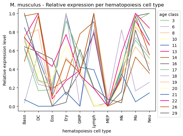
Plot relative expression per gene age class per cell type
[34]:
paul15_rematrix_grouped = orthomap2tei.get_rematrix(
    adata=paul15,
    gene_id=query_orthomap['geneNAME'],
    gene_age=query_orthomap['PSnum'],
    keep='min',
    layer=None,
    use='counts',
    var_type='mean',
    group_by_obs='cell_type',
    obs_fillna='__NaN',
    obs_type='mean',
    standard_scale=0,
    normalize_total=True,
    log1p=True,
    target_sum=1e6)
paul15_rematrix_grouped
[34]:
| cell_type | Baso | DC | Eos | Ery | GMP | Lymph | MEP | Mk | Mo | Neu |
|---|---|---|---|---|---|---|---|---|---|---|
| ps | ||||||||||
| 3 | 0.615039 | 0.167359 | 0.178835 | 1.000000 | 0.352897 | 0.000000 | 0.036377 | 0.373524 | 0.709971 | 0.517142 |
| 6 | 0.628194 | 0.236375 | 0.198174 | 1.000000 | 0.343005 | 0.000000 | 0.035514 | 0.396302 | 0.738885 | 0.560596 |
| 8 | 0.699730 | 0.277642 | 0.180843 | 1.000000 | 0.388863 | 0.003901 | 0.000000 | 0.350501 | 0.854512 | 0.653597 |
| 10 | 0.713704 | 0.308461 | 0.229101 | 1.000000 | 0.377608 | 0.007057 | 0.000000 | 0.480066 | 0.872604 | 0.730671 |
| 11 | 0.844724 | 0.517196 | 0.129400 | 0.989336 | 0.419327 | 0.393205 | 0.000000 | 0.407798 | 1.000000 | 0.708744 |
| 13 | 0.742205 | 1.000000 | 0.078693 | 0.274903 | 0.387866 | 0.782465 | 0.000000 | 0.317121 | 0.920760 | 0.660845 |
| 14 | 0.971625 | 1.000000 | 0.187126 | 0.290612 | 0.778844 | 0.909515 | 0.000000 | 0.298576 | 0.967717 | 0.553341 |
| 16 | 0.640491 | 0.583502 | 0.509405 | 0.121767 | 0.373026 | 0.802505 | 0.000000 | 0.156255 | 0.970238 | 1.000000 |
| 17 | 0.729319 | 0.279619 | 0.232445 | 0.916531 | 0.562699 | 0.191023 | 0.000000 | 0.426007 | 0.915294 | 1.000000 |
| 18 | 0.034993 | 0.574783 | 0.163902 | 1.000000 | 0.000000 | 0.827045 | 0.067891 | 0.822250 | 0.164334 | 0.258132 |
| 19 | 0.759602 | 0.824711 | 0.000000 | 0.523941 | 0.349168 | 1.000000 | 0.094374 | 0.321299 | 0.640921 | 0.451999 |
| 20 | 0.773668 | 0.373523 | 0.290813 | 0.651809 | 0.364964 | 0.016123 | 0.000000 | 0.279758 | 1.000000 | 0.798367 |
| 21 | 0.071850 | 0.000000 | 0.000000 | 0.152816 | 0.000000 | 1.000000 | 0.000000 | 0.347615 | 0.047269 | 0.143393 |
| 22 | 0.740743 | 0.550511 | 0.428294 | 0.772036 | 0.334820 | 0.191008 | 0.000000 | 0.575763 | 1.000000 | 0.841191 |
| 26 | 0.483313 | 0.968952 | 0.104028 | 0.504886 | 0.357192 | 1.000000 | 0.000000 | 0.068826 | 0.529742 | 0.355046 |
| 29 | 1.000000 | 0.466556 | 0.000000 | 0.041245 | 0.611573 | 0.200193 | 0.076297 | 0.036560 | 0.818541 | 0.384647 |
[35]:
ax = sns.lineplot(paul15_rematrix_grouped.transpose(), palette='Accent', dashes=False)
ax.legend(fontsize=5, title='age class')
ax.set_title('M. musculus - Relative expression per hematopoiesis cell type')
ax.set_xlabel('hematopoiesis cell type')
ax.set_ylabel('Relative expression level')
sns.move_legend(ax, 'upper left', bbox_to_anchor=(1, 1))
#plt.tick_params(labelsize=3)
plt.xticks(rotation=90)
plt.show()
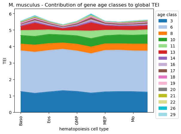
Get partial TEI values to visualize gene age class contributions
Partial TEI values can give an idea about which gene age class contributed at most to the global TEI pattern.
In detail, each gene gets a TEI contribution profile as follows:
\({TEI_{is} = f_{is} * ps_i}\)
, where \({TEI_{is}}\) is the partial TEI value of gene \({i}\), \({f_{is} = e_{is} / \sum e_{is}}\) and \({ps_i}\) is the phylostratum of gene i.
\({TEI_{is}}\) values are combined per \({ps}\).
The partial TEI values combined per strata give an overall impression of the contribution of each strata to the global TEI pattern.
One can either start from counts (adata.X) which is set as default or any other layer defined by the layer option (layer=None).
In addition, the counts can be normalized and log-transformed prior calculating partial TEI values (normalize_total=False, log1p=False, target_sum=1e6).
Further, these values can be combined per given observation, e.g. cell typer per sample timepoint (group_by='cell_state').
The get_pstrata function of the orthomap2tei submodule will return two matrix, the first contains the sum of each partial TEI per gene age class and the second the corresponding frequencies.
Both can be further processed by returning the cumsum over the gene age classes. To get them set the option cumsum=True. The cumsum will result in either for the first matrix the TEI value per cell or mean TEI value per group, if one choose a observation with the group_by option. Or in case of the second frequency matrix will result in 1.
With the standard_scale option either gene age classes (standard_scale=0 rows) or cells or groups (standard_scale=1 columns) can be scaled, subtract the minimum and divide each by its maximum. By default no scaling is applied (standard_scale=None).
The resulting data will be visualized in the downstream section.
[36]:
paul15_pstrata = orthomap2tei.get_pstrata(adata=paul15,
    gene_id=query_orthomap['geneNAME'],
    gene_age=query_orthomap['PSnum'],
    keep='min',
    layer=None,
    cumsum=False,
    group_by_obs='cell_type',
    obs_fillna='__NaN',
    obs_type='mean',
    standard_scale=None,
    normalize_total=True,
    log1p=True,
    target_sum=1e6)
paul15_pstrata[0]
[36]:
| cell_type | Baso | DC | Eos | Ery | GMP | Lymph | MEP | Mk | Mo | Neu |
|---|---|---|---|---|---|---|---|---|---|---|
| ps | ||||||||||
| 3 | 1.255834 | 1.148338 | 1.233771 | 1.310048 | 1.262417 | 1.161642 | 1.236535 | 1.254041 | 1.249693 | 1.221387 |
| 6 | 2.480437 | 2.502566 | 2.522931 | 2.517643 | 2.462211 | 2.396045 | 2.523230 | 2.519323 | 2.481219 | 2.503882 |
| 8 | 0.411742 | 0.434993 | 0.419678 | 0.386126 | 0.413464 | 0.409350 | 0.401669 | 0.391083 | 0.416381 | 0.423759 |
| 10 | 0.519061 | 0.523463 | 0.558027 | 0.488053 | 0.509677 | 0.508627 | 0.494315 | 0.535641 | 0.533390 | 0.563985 |
| 11 | 0.301539 | 0.378470 | 0.272956 | 0.253081 | 0.304966 | 0.463461 | 0.331846 | 0.288934 | 0.295967 | 0.298528 |
| 13 | 0.244590 | 0.433666 | 0.228817 | 0.141298 | 0.252155 | 0.497386 | 0.273134 | 0.230809 | 0.246127 | 0.249142 |
| 14 | 0.044808 | 0.071361 | 0.039175 | 0.022380 | 0.052420 | 0.085155 | 0.043136 | 0.037238 | 0.041165 | 0.037326 |
| 16 | 0.050629 | 0.077074 | 0.071406 | 0.027087 | 0.054985 | 0.108249 | 0.058365 | 0.041914 | 0.053758 | 0.064512 |
| 17 | 0.082491 | 0.091259 | 0.084651 | 0.073984 | 0.097491 | 0.111185 | 0.087944 | 0.083058 | 0.084383 | 0.104090 |
| 18 | 0.007005 | 0.020789 | 0.010993 | 0.014049 | 0.008381 | 0.035249 | 0.013827 | 0.020053 | 0.007336 | 0.009939 |
| 19 | 0.019848 | 0.031870 | 0.002873 | 0.011493 | 0.014289 | 0.053635 | 0.010245 | 0.012994 | 0.016351 | 0.014169 |
| 20 | 0.078326 | 0.083061 | 0.067107 | 0.053517 | 0.066933 | 0.056529 | 0.054852 | 0.056434 | 0.086404 | 0.085647 |
| 21 | 0.000092 | 0.000000 | 0.000000 | 0.000103 | 0.000000 | 0.002859 | 0.000000 | 0.000183 | 0.000060 | 0.000194 |
| 22 | 0.010988 | 0.011637 | 0.015828 | 0.008569 | 0.007818 | 0.007517 | 0.003262 | 0.010725 | 0.013529 | 0.013286 |
| 26 | 0.022055 | 0.067426 | 0.012997 | 0.016827 | 0.022783 | 0.086933 | 0.007268 | 0.008683 | 0.022500 | 0.018088 |
| 29 | 0.013402 | 0.007264 | 0.000000 | 0.000478 | 0.009943 | 0.005890 | 0.002479 | 0.000404 | 0.009816 | 0.005076 |
[37]:
#plt.rcParams['figure.figsize'] = [9, 4.5]
ax=paul15_pstrata[0].transpose().plot.area(cmap='tab20')
ax.legend(fontsize=3, title='age class')
ax.set_title('M. musculus - Contribution of gene age classes to global TEI')
ax.set_xlabel('hematopoiesis cell type')
ax.set_ylabel('TEI')
sns.move_legend(ax, 'upper left', bbox_to_anchor=(1, 1))
plt.xticks(rotation=90)
plt.show()
#plt.rcParams['figure.figsize'] = [6, 4.5]
Color UMAP/TSNE by TEI
Follwoing the tutorial of CellOracle (Kamimoto et al., 2023), one can highlight TEI values on a dimensional reduction of the scRNA dataset, like PCA, UMAP or TSNE.
Filtering
[38]:
# Only consider genes with more than 1 count
sc.pp.filter_genes(paul15, min_counts=1)
Normalization
[39]:
# Normalize gene expression matrix with total UMI count per cell
sc.pp.normalize_per_cell(paul15, key_n_counts='n_counts_all')
Identification of highly variable genes
Removing non-variable genes reduces the calculation time during the GRN reconstruction and simulation steps. It also improves the overall accuracy of the GRN inference by removing noisy genes. We recommend using the top 2000~3000 variable genes.
[40]:
# Select top 2000 highly-variable genes
filter_result = sc.pp.filter_genes_dispersion(paul15.X,
                                              flavor='cell_ranger',
                                              n_top_genes=2000,
                                              log=False)

# Subset the genes
paul15 = paul15[:, filter_result.gene_subset]

# Renormalize after filtering
sc.pp.normalize_per_cell(paul15)
/opt/anaconda3/envs/scanpy/lib/python3.8/site-packages/scanpy/preprocessing/_simple.py:524: ImplicitModificationWarning: Trying to modify attribute `.obs` of view, initializing view as actual.
  adata.obs[key_n_counts] = counts_per_cell
Log transformation
We need to log transform and scale the data before we calculate the principal components, clusters, and differentially expressed genes.
We also need to keep the non-transformed gene expression data in a separate anndata layer before the log transformation. We will use this data for celloracle analysis later.
[41]:
# keep raw cont data before log transformation
paul15.raw = paul15
paul15.layers["raw_count"] = paul15.raw.X.copy()

# Log transformation and scaling
sc.pp.log1p(paul15)
sc.pp.scale(paul15)
PCA and neighbor calculations
These calculations are necessary to perform the dimensionality reduction and clustering steps.
[42]:
# PCA
sc.tl.pca(paul15, svd_solver='arpack')

# Diffusion map
sc.pp.neighbors(paul15, n_neighbors=4, n_pcs=20)

sc.tl.diffmap(paul15)
# Calculate neihbors again based on diffusionmap
sc.pp.neighbors(paul15, n_neighbors=10, use_rep='X_diffmap')
Cell clustering
[43]:
sc.tl.louvain(paul15, resolution=0.8)
Embedding the neighborhood graph
[44]:
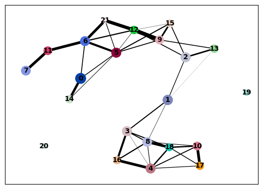
# PAGA graph construction
sc.tl.paga(paul15, groups='louvain')
[45]:
sc.pl.paga(paul15)
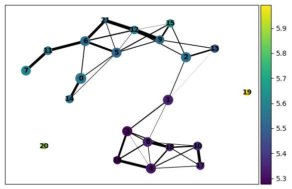
Color PAGA graph
[46]:
sc.pl.paga(paul15, color='tei')
[47]:
sc.tl.draw_graph(paul15, init_pos='paga', random_state=123)
WARNING: Package 'fa2' is not installed, falling back to layout 'fr'.To use the faster and better ForceAtlas2 layout, install package 'fa2' (`pip install fa2`).
[48]:
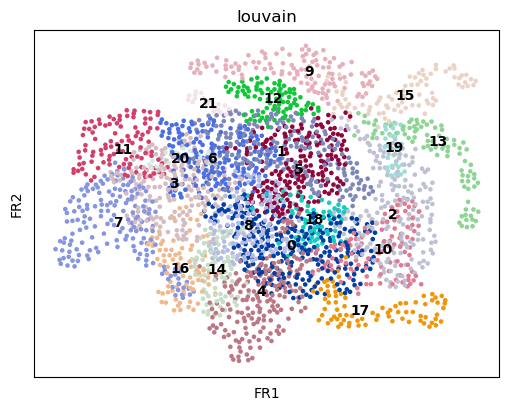
sc.pl.draw_graph(paul15, color='louvain', legend_loc='on data')
/opt/anaconda3/envs/scanpy/lib/python3.8/site-packages/scanpy/plotting/_tools/scatterplots.py:392: UserWarning: No data for colormapping provided via 'c'. Parameters 'cmap' will be ignored
  cax = scatter(
[49]:
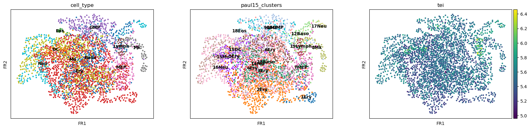
sc.pl.draw_graph(paul15, color=['cell_type', 'paul15_clusters', 'tei'],
                 legend_loc='on data')
/opt/anaconda3/envs/scanpy/lib/python3.8/site-packages/scanpy/plotting/_tools/scatterplots.py:392: UserWarning: No data for colormapping provided via 'c'. Parameters 'cmap' will be ignored
  cax = scatter(
/opt/anaconda3/envs/scanpy/lib/python3.8/site-packages/scanpy/plotting/_tools/scatterplots.py:392: UserWarning: No data for colormapping provided via 'c'. Parameters 'cmap' will be ignored
  cax = scatter(
UMAP
[50]:
sc.tl.umap(paul15,
init_pos='paga')
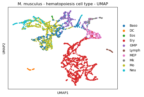
sc.pl.umap(paul15,
title='M. musculus - hematopoiesis cell type - UMAP', color=['cell_type'])
/opt/anaconda3/envs/scanpy/lib/python3.8/site-packages/scanpy/plotting/_tools/scatterplots.py:392: UserWarning: No data for colormapping provided via 'c'. Parameters 'cmap' will be ignored
  cax = scatter(
[51]:
#plt.rcParams['figure.figsize'] = [7.5, 4.5]
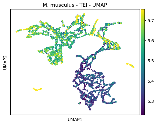
sc.pl.umap(paul15,
title='M. musculus - TEI - UMAP',
color=['tei'],
color_map='viridis',
vmin='p5',
vmax='p95')
#plt.rcParams['figure.figsize'] = [6, 4.5]
[52]:
#3d
sc.tl.umap(paul15,
           n_components=3)
sc.pl.umap(paul15,
           title='M. musculus - hematopoiesis cell type - UMAP', color=['cell_type'],
           projection='3d')
/opt/anaconda3/envs/scanpy/lib/python3.8/site-packages/scanpy/plotting/_tools/scatterplots.py:325: UserWarning: No data for colormapping provided via 'c'. Parameters 'cmap' will be ignored
  cax = ax.scatter(
[53]:
#plt.rcParams['figure.figsize'] = [7.5, 4.5]
sc.pl.umap(paul15,
           title='M. musculus - TEI - UMAP',
           color=['tei'],
           color_map='viridis',
           vmin='p5',
           vmax='p95',
           projection='3d')
#plt.rcParams['figure.figsize'] = [6, 4.5]

[54]:
import plotly
import kaleido
import plotly.express as px
plotly.offline.init_notebook_mode(connected=False)
[55]:
df = pd.DataFrame( {'UMAP1':paul15.obsm['X_umap'][:,0],
                    'UMAP2':paul15.obsm['X_umap'][:,1],
                    'UMAP3':paul15.obsm['X_umap'][:,2],
                    'cell_type':paul15.obs['cell_type'].values.astype(str),
                    'tei':paul15.obs['tei'].values,
                    'cell_id':paul15.obs.index.to_list()  } )
df.set_index('cell_id', inplace = True)
df.head()
[55]:
| UMAP1 | UMAP2 | UMAP3 | cell_type | tei | |
|---|---|---|---|---|---|
| cell_id | |||||
| 0 | 11.113059 | 7.795863 | -0.662884 | MEP | 5.420982 |
| 1 | 16.109194 | 0.734038 | 11.387341 | Mo | 5.598349 |
| 2 | 3.196870 | -5.445777 | 6.057778 | Ery | 5.361106 |
| 3 | 13.342421 | 0.143536 | 4.945064 | Mo | 5.551194 |
| 4 | 3.316909 | -3.929081 | 6.646379 | Ery | 5.362875 |
[56]:
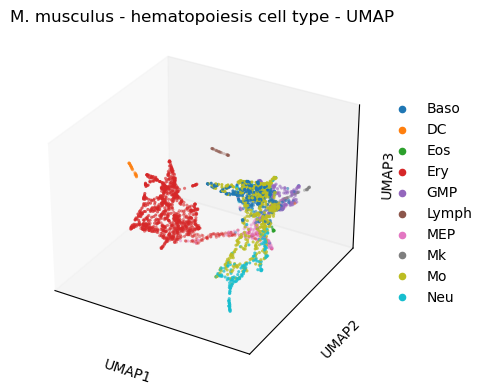
fig = px.scatter_3d(data_frame = df,
                    x='UMAP1',
                    y='UMAP2',
                    z='UMAP3',
                    color='cell_type')
fig.update_traces(marker_size = 2)
fig.write_html('mouse_scatter_3d_cell_type.html')
[57]:
fig = px.scatter_3d(data_frame = df,
                    x='UMAP1',
                    y='UMAP2',
                    z='UMAP3',
                    color='tei',
                    range_color=(5,5.5))
fig.update_traces(marker_size = 2)
fig.write_html('mouse_scatter_3d_tei.html')
Please have a look at the documentation for other case studies.