Case study: re-analysis of zebrafish (Danio rerio) embryogenesis single-cell data
This notebook will demonstrate scRNA-seq processing with oggmap using zebrafish scRNA data from (Farrell et al., 2018; Wagner et al., 2018; Qiu et al., 2022).
scRNA data were obtained from http://tome.gs.washington.edu/, converted into Scanpy AnnData objects (Wolf et al., 2018) and are availabe here:
https://doi.org/10.5281/zenodo.7243602
or can be accessed with the dataset submodule of oggmap
datasets.qiu22_zebrafish(datapath='data') (download folder set to 'data').
Notebook file
Notebook file can be obtained here:
https://raw.githubusercontent.com/kullrich/oggmap/main/docs/notebooks/zebrafish_example.ipynb
Steps
To process the scRNA data, we will do the following:
Run OrthoFinder to obtain orthogroups
Get query species taxonomic lineage information
Get query species orthomap
Map OrthoFinder gene names and scRNA gene/transcript names
Get TEI values and add them to scRNA dataset
Get partial TEI values to visualize gene age class contributions
Process scRNA data and visualize TEI
Import libraries
[1]:
import numpy as np
import pandas as pd
import scanpy as sc
import seaborn as sns
import matplotlib.pyplot as plt
from statannot import add_stat_annotation
# increase dpi
%matplotlib inline
#plt.rcParams['figure.dpi'] = 300
#plt.rcParams['savefig.dpi'] = 300
#plt.rcParams['figure.figsize'] = [6, 4.5]
plt.rcParams['figure.figsize'] = [4.4, 3.3]
Import oggmap python package submodules
[2]:
# import submodules
from oggmap import qlin, gtf2t2g, of2orthomap, orthomap2tei, datasets
Step 0 - run OrthoFinder to obtain orthogroups
oggmap can extract gene age classification from existing OrthoFinder results and link them with scRNA data.
A detailed how-to is available here:
https://oggmap.readthedocs.io/en/latest/tutorials/orthofinder.html
However, any pre-calculated gene age classification can be imported as a table using the function orthomap2tei.read_orthomap(orthomapfile=filename).
The pre-calculated gene age classification file should be delimited with two columns GeneID<tab>Phylostratum, like e.g.:
GeneID<tab>Phylostratum
WBGene00000001<tab>1
WBGene00000002<tab>1
WBGene00000003<tab>1
WBGene00000004<tab>1
WBGene00000005<tab>2
OrthoFinder (Emms and Kelly, 2019) results (-S last) using translated, longest-isoform coding sequences (CDS) from Ensembl release-110, including species taxonomic IDs, are available here:
https://doi.org/10.5281/zenodo.7242264
or can be accessed with the dataset submodule of oggmap
datasets.ensembl110_last(datapath='data') (download folder set to 'data').
[3]:
datasets.ensembl110_last(datapath='data')
99% [..................................................... ] 1318912 / 1325809100% [..........................................................] 11317 / 11317
[3]:
['data/ensembl_110_orthofinder_last_Orthogroups.GeneCount.tsv.zip',
 'data/ensembl_110_orthofinder_last_Orthogroups.tsv.zip',
 'data/ensembl_110_orthofinder_last_species_list.tsv']
Step 1 - get query species taxonomic lineage information
Given a species name or taxonomic ID, the query species lineage information is extracted with the help of the ete3 python toolkit and the NCBI taxonomy (Huerta-Cepas et al., 2016). This information is needed alongside with the taxonomic classifications for all species used in the OrthoFinder comparison.
The oggmap submodule qlin helps to get this information for you with the qlin.get_qlin() function as follows:
[4]:
# get query species taxonomic lineage information
query_lineage = qlin.get_qlin(q='Danio rerio')
query name: Danio rerio
query taxID: 7955
query kingdom: Eukaryota
query lineage names:
['root(1)', 'cellular organisms(131567)', 'Eukaryota(2759)', 'Opisthokonta(33154)', 'Metazoa(33208)', 'Eumetazoa(6072)', 'Bilateria(33213)', 'Deuterostomia(33511)', 'Chordata(7711)', 'Craniata(89593)', 'Vertebrata(7742)', 'Gnathostomata(7776)', 'Teleostomi(117570)', 'Euteleostomi(117571)', 'Actinopterygii(7898)', 'Actinopteri(186623)', 'Neopterygii(41665)', 'Teleostei(32443)', 'Osteoglossocephalai(1489341)', 'Clupeocephala(186625)', 'Otomorpha(186634)', 'Ostariophysi(32519)', 'Otophysi(186626)', 'Cypriniphysae(186627)', 'Cypriniformes(7952)', 'Cyprinoidei(30727)', 'Danionidae(2743709)', 'Danioninae(2743711)', 'Danio(7954)', 'Danio rerio(7955)']
query lineage:
[1, 131567, 2759, 33154, 33208, 6072, 33213, 33511, 7711, 89593, 7742, 7776, 117570, 117571, 7898, 186623, 41665, 32443, 1489341, 186625, 186634, 32519, 186626, 186627, 7952, 30727, 2743709, 2743711, 7954, 7955]
Step 2 - gene age class assignment (query species orthomap)
Here, oggmap use the query species information and OrthoFinder results to extract the oldest common tree node per orthogroup along a species tree and to assign this node as the gene age to the corresponding genes.
In a pairwise manner, the query species and any other species in the OrthoFinder result might share multiple tree nodes down to the root of the species tree, but have only one youngest tree node in common. Among all possible comparison between the query species and the other species, the oldest as defined by the species tree root is seected and used for the gene age assignment.
Given the query species sequence name (seqname=) used in the OrthoFinder comparison, the query species taxonomic ID(qt=), the taxonomic IDs of all species (sl=) used in the OrthoFinder comparison, the orthogroup gene count (oc=) results and the orthogroups (og=), an orthomap is constructed.
Note: This step can take up to five minutes, depending on your hardware.
For this step to get the query species orthomap, one uses the of2orthomap.get_orthomap() function, like:
corresponds to main figure Figure 1B
[5]:
# get query species orthomap

# download orthofinder results here: https://doi.org/10.5281/zenodo.7242264
# or download with datasets.ensembl110_last('data')
query_orthomap, orthofinder_species_list, of_species_abundance = of2orthomap.get_orthomap(
    seqname='7955.danio_rerio.pep',
    qt='7955',
    sl='data/ensembl_110_orthofinder_last_species_list.tsv',
    oc='data/ensembl_110_orthofinder_last_Orthogroups.GeneCount.tsv.zip',
    og='data/ensembl_110_orthofinder_last_Orthogroups.tsv.zip',
    continuity=True)
query_orthomap
7955.danio_rerio.pep
Danio rerio
7955
                                    species  taxID  \
0                 10020.dipodomys_ordii.pep  10020
1    10029.cricetulus_griseus_chok1gshd.pep  10029
2       10029.cricetulus_griseus_crigri.pep  10029
3         10029.cricetulus_griseus_picr.pep  10029
4            10036.mesocricetus_auratus.pep  10036
..                                      ...    ...
313          9986.oryctolagus_cuniculus.pep   9986
314        99883.tetraodon_nigroviridis.pep  99883
315        9994.marmota_marmota_marmota.pep   9994
316            9999.urocitellus_parryii.pep   9999
317    Xtropicalisv9.0.Named.primaryTrs.pep   8364

                                               lineage  youngest_common  \
0    [1, 131567, 2759, 33154, 33208, 6072, 33213, 3...           117571
1    [1, 131567, 2759, 33154, 33208, 6072, 33213, 3...           117571
2    [1, 131567, 2759, 33154, 33208, 6072, 33213, 3...           117571
3    [1, 131567, 2759, 33154, 33208, 6072, 33213, 3...           117571
4    [1, 131567, 2759, 33154, 33208, 6072, 33213, 3...           117571
..                                                 ...              ...
313  [1, 131567, 2759, 33154, 33208, 6072, 33213, 3...           117571
314  [1, 131567, 2759, 33154, 33208, 6072, 33213, 3...           186625
315  [1, 131567, 2759, 33154, 33208, 6072, 33213, 3...           117571
316  [1, 131567, 2759, 33154, 33208, 6072, 33213, 3...           117571
317  [1, 131567, 2759, 33154, 33208, 6072, 33213, 3...           117571

     youngest_name
0     Euteleostomi
1     Euteleostomi
2     Euteleostomi
3     Euteleostomi
4     Euteleostomi
..             ...
313   Euteleostomi
314  Clupeocephala
315   Euteleostomi
316   Euteleostomi
317   Euteleostomi

[318 rows x 5 columns]
[5]:
| seqID | Orthogroup | PSnum | PStaxID | PSname | PScontinuity | |
|---|---|---|---|---|---|---|
| 0 | ENSDART00000013359.10 | OG0000000 | 6 | 33213 | Bilateria | 0.846154 |
| 1 | ENSDART00000136092.3 | OG0000001 | 6 | 33213 | Bilateria | 1.000000 |
| 2 | ENSDART00000148349.3 | OG0000001 | 6 | 33213 | Bilateria | 1.000000 |
| 3 | ENSDART00000160249.2 | OG0000001 | 6 | 33213 | Bilateria | 1.000000 |
| 4 | ENSDART00000174091.2 | OG0000001 | 6 | 33213 | Bilateria | 1.000000 |
| ... | ... | ... | ... | ... | ... | ... |
| 24952 | ENSDART00000125904.3 | OG0035492 | 19 | 186625 | Clupeocephala | 0.400000 |
| 24953 | ENSDART00000191935.1 | OG0035493 | 25 | 30727 | Cyprinoidei | 1.000000 |
| 24954 | ENSDART00000143229.2 | OG0035494 | 29 | 7955 | Danio rerio | 1.000000 |
| 24955 | ENSDART00000143837.3 | OG0035494 | 29 | 7955 | Danio rerio | 1.000000 |
| 24956 | ENSDART00000143384.2 | OG0035495 | 22 | 186626 | Otophysi | 0.666667 |
24957 rows × 6 columns
Gene age assignments per query species lineage node
Given an orthomap, one can get an overview of the gene age assignments per query species lineage node.
The oggmap submodule of2orhomap and the of2orthomap.get_counts_per_ps() function will show the distribution of the gene age classes and can be further visualized as follows:
[6]:
# show count per taxonomic group (PStaxID)
of2orthomap.get_counts_per_ps(query_orthomap)
[6]:
| PSnum | counts | PStaxID | PSname | |
|---|---|---|---|---|
| PSnum | ||||
| 3 | 3 | 4376 | 33154 | Opisthokonta |
| 6 | 6 | 10530 | 33213 | Bilateria |
| 8 | 8 | 2390 | 7711 | Chordata |
| 10 | 10 | 2838 | 7742 | Vertebrata |
| 11 | 11 | 1515 | 7776 | Gnathostomata |
| 13 | 13 | 760 | 117571 | Euteleostomi |
| 14 | 14 | 235 | 7898 | Actinopterygii |
| 16 | 16 | 275 | 41665 | Neopterygii |
| 18 | 18 | 231 | 1489341 | Osteoglossocephalai |
| 19 | 19 | 506 | 186625 | Clupeocephala |
| 20 | 20 | 33 | 186634 | Otomorpha |
| 22 | 22 | 120 | 186626 | Otophysi |
| 25 | 25 | 317 | 30727 | Cyprinoidei |
| 29 | 29 | 831 | 7955 | Danio rerio |
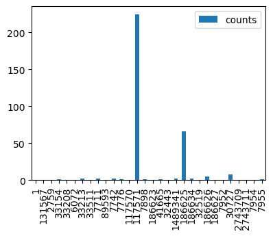
Visualize number of species along query lineage and counts per gene age class
[7]:
# show number of species along query lineage
of_species_abundance

# bar plot number of species along query lineage
of_species_abundance.plot.bar(y='counts', use_index=True)
[7]:
<AxesSubplot: >
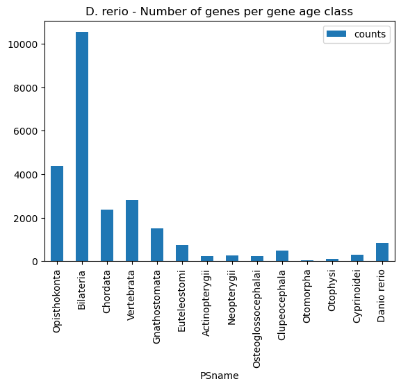
corresponds to main figure Figure 1C
[8]:
plt.rcParams['figure.figsize'] = [6.5, 4.5]
# show count per taxonomic group (PStaxID)
of2orthomap.get_counts_per_ps(query_orthomap)

# bar plot count per taxonomic group (PSname)
ax = of2orthomap.get_counts_per_ps(query_orthomap).plot.bar(y='counts', x='PSname')
ax.set_title('D. rerio - Number of genes per gene age class')
plt.show()
plt.rcParams['figure.figsize'] = [4.4, 3.3]
Step 3 - map OrthoFinder gene names and scRNA gene/transcript names
To be able to link gene ages assignments from an orthomap and gene or transcript of scRNA dataset, one needs to check the overlap of the annotated gene names. With the gtf2t2g submodule of oggmap and the gtf2t2g.parse_gtf() function, one can extract gene and transcript names from a given gene feature file (GTF).
[9]:
datasets.zebrafish_ensembl110_gtf('data')
100% [....................................................] 18055420 / 18055420
[9]:
'data/Danio_rerio.GRCz11.110.gtf.gz'
[10]:
# get gene to transcript table for Danio rerio

# download zebrafish GTF file here:
# https://ftp.ensembl.org/pub/release-110/gtf/danio_rerio/Danio_rerio.GRCz11.110.gtf.gz
# or download with datasets.zebrafish_ensembl110_gtf('data')
query_species_t2g = gtf2t2g.parse_gtf(
    gtf='data/Danio_rerio.GRCz11.110.gtf.gz',
    g=True, b=True, p=True, v=True, s=True, q=True)
32520 gene_id found
59876 transcript_id found
59876 protein_id found
0 duplicated
[11]:
query_species_t2g
[11]:
| gene_id | gene_id_version | transcript_id | transcript_id_version | gene_name | gene_type | protein_id | protein_id_version | |
|---|---|---|---|---|---|---|---|---|
| 0 | ENSDARG00000000001 | ENSDARG00000000001.6 | ENSDART00000000004 | ENSDART00000000004.5 | slc35a5 | protein_coding | ENSDARP00000000004 | ENSDARP00000000004.2 |
| 1 | ENSDARG00000000002 | ENSDARG00000000002.8 | ENSDART00000000005 | ENSDART00000000005.7 | ccdc80 | protein_coding | ENSDARP00000000005 | ENSDARP00000000005.6 |
| 2 | ENSDARG00000000018 | ENSDARG00000000018.9 | ENSDART00000181044 | ENSDART00000181044.1 | nrf1 | protein_coding | ENSDARP00000149440 | ENSDARP00000149440.1 |
| 3 | ENSDARG00000000018 | ENSDARG00000000018.9 | ENSDART00000138183 | ENSDART00000138183.2 | nrf1 | protein_coding | ENSDARP00000116798 | ENSDARP00000116798.1 |
| 4 | ENSDARG00000000019 | ENSDARG00000000019.9 | ENSDART00000124452 | ENSDART00000124452.3 | ube2h | protein_coding | ENSDARP00000107407 | ENSDARP00000107407.2 |
| ... | ... | ... | ... | ... | ... | ... | ... | ... |
| 59871 | ENSDARG00000117825 | ENSDARG00000117825.1 | ENSDART00000194739 | ENSDART00000194739.1 | None | lincRNA | None | None |
| 59872 | ENSDARG00000117826 | ENSDARG00000117826.1 | ENSDART00000194042 | ENSDART00000194042.1 | None | lincRNA | None | None |
| 59873 | ENSDARG00000117826 | ENSDARG00000117826.1 | ENSDART00000194514 | ENSDART00000194514.1 | None | lincRNA | None | None |
| 59874 | ENSDARG00000117827 | ENSDARG00000117827.1 | ENSDART00000194378 | ENSDART00000194378.1 | None | lincRNA | None | None |
| 59875 | ENSDARG00000117827 | ENSDARG00000117827.1 | ENSDART00000194710 | ENSDART00000194710.1 | None | lincRNA | None | None |
59876 rows × 8 columns
Import now, the scRNA dataset of the query species
Here, data is used, like in the publication (Farrell et al., 2018; Wagner et al., 2018; Qiu et al., 2022).
scRNA data was downloaded from http://tome.gs.washington.edu/ as R rds files, combined into a single Seurat object and converted into loom and AnnData (h5ad) files to be able to analyse with e.g. python scanpy or oggmap package and is available here:
https://doi.org/10.5281/zenodo.7243602
or can be accessed with the dataset submodule of oggmap:
datasets.qiu22_zebrafish(datapath='data') (download folder set to 'data').
[12]:
# load scRNA data

# download zebrafish scRNA data here: https://doi.org/10.5281/zenodo.7243602
# or download with datasets.qui22_zebrafish(datapath='data')

#zebrafish_data = datasets.qiu22_zebrafish(datapath='data')
zebrafish_data = sc.read('data/zebrafish_data.h5ad')
Get an overview of observations
[13]:
zebrafish_data
[13]:
AnnData object with n_obs × n_vars = 71203 × 20418
    obs: 'orig.ident', 'nCount_RNA', 'nFeature_RNA', 'sample', 'stage', 'group', 'cell_state', 'cell_type'
    var: 'features', 'genes'
[14]:
zebrafish_data.obs
[14]:
| orig.ident | nCount_RNA | nFeature_RNA | sample | stage | group | cell_state | cell_type | |
|---|---|---|---|---|---|---|---|---|
| hpf3.3_ZFHIGH_WT_DS5_AAAAGTTGCCTC | ZFHIGH | 5773.0 | 2570 | ZFHIGH_WT_DS5_AAAAGTTGCCTC | hpf3.3 | F_3.3 | hpf3.3:blastomere | blastomere |
| hpf3.3_ZFHIGH_WT_DS5_AAACAAGTGTAT | ZFHIGH | 2312.0 | 1451 | ZFHIGH_WT_DS5_AAACAAGTGTAT | hpf3.3 | F_3.3 | hpf3.3:blastomere | blastomere |
| hpf3.3_ZFHIGH_WT_DS5_AAACACCTCGTC | ZFHIGH | 4180.0 | 2166 | ZFHIGH_WT_DS5_AAACACCTCGTC | hpf3.3 | F_3.3 | hpf3.3:blastomere | blastomere |
| hpf3.3_ZFHIGH_WT_DS5_AAATGAGGTTTN | ZFHIGH | 6686.0 | 2845 | ZFHIGH_WT_DS5_AAATGAGGTTTN | hpf3.3 | F_3.3 | hpf3.3:blastomere | blastomere |
| hpf3.3_ZFHIGH_WT_DS5_AACCCTCTCGAT | ZFHIGH | 20095.0 | 4993 | ZFHIGH_WT_DS5_AACCCTCTCGAT | hpf3.3 | F_3.3 | hpf3.3:blastomere | blastomere |
| ... | ... | ... | ... | ... | ... | ... | ... | ... |
| hpf24_DEW057_TGACACAACAG_GCCACATC | DEW057 | 3916.0 | 1328 | DEW057_TGACACAACAG_GCCACATC | hpf24 | batch2 | hpf24:midbrain | midbrain |
| hpf24_DEW057_CTTACGGG_AACCTGAC | DEW057 | 5611.0 | 1700 | DEW057_CTTACGGG_AACCTGAC | hpf24 | batch2 | hpf24:pharyngeal arch | pharyngeal arch |
| hpf24_DEW057_TGAACATCTAT_GACGATGG | DEW057 | 3676.0 | 1345 | DEW057_TGAACATCTAT_GACGATGG | hpf24 | batch2 | hpf24:midbrain | midbrain |
| hpf24_DEW057_TGAGGTTTCTC_CTCAGAAT | DEW057 | 7021.0 | 1778 | DEW057_TGAGGTTTCTC_CTCAGAAT | hpf24 | batch2 | hpf24:optic cup | optic cup |
| hpf24_DEW057_ACGTGCTAG_CAAGTCAT | DEW057 | 3378.0 | 1170 | DEW057_ACGTGCTAG_CAAGTCAT | hpf24 | batch2 | hpf24:hindbrain dorsal | hindbrain dorsal |
71203 rows × 8 columns
Helper functions to match gene names
The orthomap2tei submodule contains the orthomap2tei.geneset_overlap() helper function to check for gene name overlap between the constructed orthomap from OrthoFinder results and a given scRNA dataset.
[15]:
# check overlap of orthomap <seqID> and scRNA data <var_names>
orthomap2tei.geneset_overlap(zebrafish_data.var_names, query_orthomap['seqID'])
[15]:
| g1_g2_overlap | g1_ratio | g2_ratio | |
|---|---|---|---|
| 0 | 0 | 0.0 | 0.0 |
[16]:
# check overlap of transcript table <gene_id> and scRNA data <var_names>
orthomap2tei.geneset_overlap(zebrafish_data.var_names, query_species_t2g['gene_id'])
[16]:
| g1_g2_overlap | g1_ratio | g2_ratio | |
|---|---|---|---|
| 0 | 20418 | 1.0 | 0.62786 |
Reduce isoforms to genes
The of2orthomap.replace_by() helper function can be used to add a new column to the orthomap dataframe by matching e.g. gene isoform names and their corresponding gene names.
[17]:
query_orthomap
[17]:
| seqID | Orthogroup | PSnum | PStaxID | PSname | PScontinuity | |
|---|---|---|---|---|---|---|
| 0 | ENSDART00000013359.10 | OG0000000 | 6 | 33213 | Bilateria | 0.846154 |
| 1 | ENSDART00000136092.3 | OG0000001 | 6 | 33213 | Bilateria | 1.000000 |
| 2 | ENSDART00000148349.3 | OG0000001 | 6 | 33213 | Bilateria | 1.000000 |
| 3 | ENSDART00000160249.2 | OG0000001 | 6 | 33213 | Bilateria | 1.000000 |
| 4 | ENSDART00000174091.2 | OG0000001 | 6 | 33213 | Bilateria | 1.000000 |
| ... | ... | ... | ... | ... | ... | ... |
| 24952 | ENSDART00000125904.3 | OG0035492 | 19 | 186625 | Clupeocephala | 0.400000 |
| 24953 | ENSDART00000191935.1 | OG0035493 | 25 | 30727 | Cyprinoidei | 1.000000 |
| 24954 | ENSDART00000143229.2 | OG0035494 | 29 | 7955 | Danio rerio | 1.000000 |
| 24955 | ENSDART00000143837.3 | OG0035494 | 29 | 7955 | Danio rerio | 1.000000 |
| 24956 | ENSDART00000143384.2 | OG0035495 | 22 | 186626 | Otophysi | 0.666667 |
24957 rows × 6 columns
[18]:
zebrafish_data.var_names
[18]:
Index(['ENSDARG00000002968', 'ENSDARG00000056314', 'ENSDARG00000102274',
       'ENSDARG00000012468', 'ENSDARG00000063621', 'ENSDARG00000044802',
       'ENSDARG00000011410', 'ENSDARG00000041170', 'ENSDARG00000011855',
       'ENSDARG00000103957',
       ...
       'ENSDARG00000078476', 'ENSDARG00000058562', 'ENSDARG00000110745',
       'ENSDARG00000114172', 'ENSDARG00000110433', 'ENSDARG00000098193',
       'ENSDARG00000101137', 'ENSDARG00000095817', 'ENSDARG00000079034',
       'ENSDARG00000063372'],
      dtype='object', name='index', length=20418)
[19]:
# convert orthomap transcript IDs into GeneIDs and add them to orthomap
query_orthomap['geneID'] = orthomap2tei.replace_by(
    x_orig = query_orthomap['seqID'],
    xmatch = query_species_t2g['transcript_id_version'],
    xreplace = query_species_t2g['gene_id'],
)
[20]:
query_orthomap
[20]:
| seqID | Orthogroup | PSnum | PStaxID | PSname | PScontinuity | geneID | |
|---|---|---|---|---|---|---|---|
| 0 | ENSDART00000013359.10 | OG0000000 | 6 | 33213 | Bilateria | 0.846154 | ENSDARG00000013014 |
| 1 | ENSDART00000136092.3 | OG0000001 | 6 | 33213 | Bilateria | 1.000000 | ENSDARG00000100568 |
| 2 | ENSDART00000148349.3 | OG0000001 | 6 | 33213 | Bilateria | 1.000000 | ENSDARG00000094216 |
| 3 | ENSDART00000160249.2 | OG0000001 | 6 | 33213 | Bilateria | 1.000000 | ENSDARG00000099070 |
| 4 | ENSDART00000174091.2 | OG0000001 | 6 | 33213 | Bilateria | 1.000000 | ENSDARG00000105690 |
| ... | ... | ... | ... | ... | ... | ... | ... |
| 24952 | ENSDART00000125904.3 | OG0035492 | 19 | 186625 | Clupeocephala | 0.400000 | ENSDARG00000110323 |
| 24953 | ENSDART00000191935.1 | OG0035493 | 25 | 30727 | Cyprinoidei | 1.000000 | ENSDARG00000114540 |
| 24954 | ENSDART00000143229.2 | OG0035494 | 29 | 7955 | Danio rerio | 1.000000 | ENSDARG00000069978 |
| 24955 | ENSDART00000143837.3 | OG0035494 | 29 | 7955 | Danio rerio | 1.000000 | ENSDARG00000078193 |
| 24956 | ENSDART00000143384.2 | OG0035495 | 22 | 186626 | Otophysi | 0.666667 | ENSDARG00000092452 |
24957 rows × 7 columns
[21]:
# check overlap of orthomap <geneID> and scRNA data
orthomap2tei.geneset_overlap(zebrafish_data.var_names, query_orthomap['geneID'])
[21]:
| g1_g2_overlap | g1_ratio | g2_ratio | |
|---|---|---|---|
| 0 | 19952 | 0.977177 | 0.799455 |
The created orthomap can be stored as a separated file like:
[22]:
query_orthomap.to_csv('./data/zebrafish_ensembl_110_orthomap.tsv', sep='\t', index=False)
To re-use the saved orthomap, so that one does not need to repeat step1 and step2, one could load it with orthomap2tei.read_orthomap() function.
Step 4 - get TEI values and add them to scRNA dataset
Since now the gene names correspond to each other in the orthomap and the scRNA adata object, one can calculate the transcriptome evolutionary index (TEI) and add them to the scRNA dataset (adata object).
The TEI measure represents the weighted arithmetic mean (expression levels as weights for the phylostratum value) over all evolutionary age categories denoted as phylostra.
\({TEI_s = \sum (e_{is} * ps_i) / \sum e_{is}}\)
, where \({TEI_s}\) denotes the TEI value in developmental stage \({s, e_{is}}\) denotes the gene expression level of gene \({i}\) in stage \({s}\), and \({ps_i}\) denotes the corresponding phylostratum of gene \({i, i = 1,...,N}\) and \({N = total\ number\ of\ genes}\).
Note: If e.g. two different isoforms would fall into two different gene age classes, their gene ages might differ based on the oldest ortholog found in their corresponding orthologous groups. However, both isoforms share the same gene name and their gene ages would clash. In this case one can decide either to use the keep='min' or keep='max' gene age to be kept by the get_tei function, which defaults to keep in this cases the keep='min' or in other words the ‘older’ gene age.
To be able to re-use the original count data, they are added as a new layer to the adata object. This is useful because later on the count data can be used to extract either the relative expression per gene age class or re-calculate other metrics.
This can be done either on un-normalized counts, on normalized and log-transformed data.
[23]:
zebrafish_data.layers['counts'] = zebrafish_data.X
add TEI to adata object
Using the submodule orthomap2tei from oggmap and the orthomap2tei.get_tei() function, transcriptome evolutionary index (TEI) values are calculated and directyl added to the existing adata object (add_obs=True).
There are other options to e.g. not start from the adata.X counts but from another layer from the adata object, the default is to use the adata.X (layer=None). The values can be pre-processed by the normalize_total option and the log1p option.
If add_obs=True the resulting TEI values are added to the existing adata object as a new observation with the name set with the obs_name option.
If add_var=True the gene age values are added to the existing adata object as a new variable with the name set with the var_name option.
Note: Genes not assigned to any gene class will get a missing assignment.
If one wants to calculate bootstrap TEI values per cell, the boot option can be set to boot=True and gene age classes will be randomly chosen prior calculating TEI values bt=10 times.
[24]:
# add TEI values to existing adata object
orthomap2tei.get_tei(adata=zebrafish_data,
    gene_id=query_orthomap['geneID'],
    gene_age=query_orthomap['PSnum'],
    keep='min',
    layer=None,
    add_var=True,
    var_name='Phylostrata',
    add_obs=True,
    obs_name='tei',
    boot=False,
    bt=10,
    normalize_total=True,
    log1p=True,
    target_sum=1e6)
[24]:
| tei | |
|---|---|
| hpf3.3_ZFHIGH_WT_DS5_AAAAGTTGCCTC | 5.847391 |
| hpf3.3_ZFHIGH_WT_DS5_AAACAAGTGTAT | 5.794241 |
| hpf3.3_ZFHIGH_WT_DS5_AAACACCTCGTC | 5.783182 |
| hpf3.3_ZFHIGH_WT_DS5_AAATGAGGTTTN | 5.780480 |
| hpf3.3_ZFHIGH_WT_DS5_AACCCTCTCGAT | 5.915213 |
| ... | ... |
| hpf24_DEW057_TGACACAACAG_GCCACATC | 5.429996 |
| hpf24_DEW057_CTTACGGG_AACCTGAC | 5.612010 |
| hpf24_DEW057_TGAACATCTAT_GACGATGG | 5.374328 |
| hpf24_DEW057_TGAGGTTTCTC_CTCAGAAT | 5.260610 |
| hpf24_DEW057_ACGTGCTAG_CAAGTCAT | 5.644344 |
71203 rows × 1 columns
Step 5 - downstream analysis
Once the gene age data has been added to the scRNA dataset, one can e.g. plot the corresponding transcriptome evolutionary index (TEI) values by any given observation pre-defined in the scRNA dataset.
Here, we plot them against the assigned embryo stage and against assigned cell types of the zebrafish using the scanpy sc.pl.violin() function as follows:
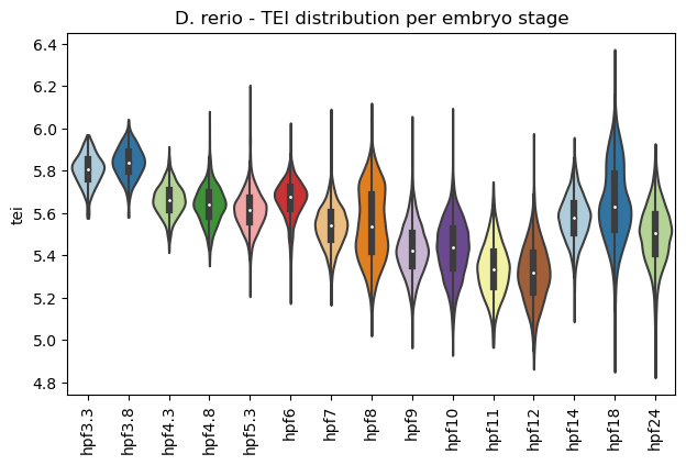
Boxplot gene age class per embryo stage
corresponds to main figure Figure 1D
[25]:
plt.rcParams['figure.figsize'] = [6.5, 4.5]
ax = sc.pl.violin(adata=zebrafish_data,
                  keys=['tei'],
                  groupby='stage',
                  rotation=90,
                  palette='Paired',
                  stripplot=False,
                  inner='box',
                  show=False)
ax.set_title('D. rerio - TEI distribution per embryo stage')
plt.show()
plt.rcParams['figure.figsize'] = [4.4, 3.3]
Boxplot gene age class per embryo stage and add significance
Note: Please change notebook cell from raw to code to see the plots.
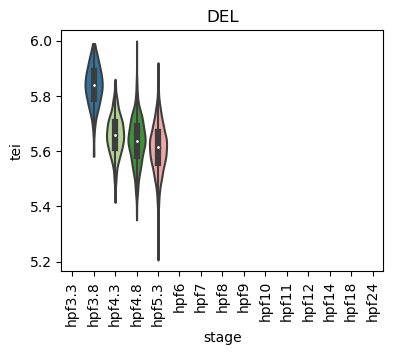
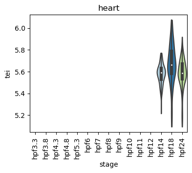
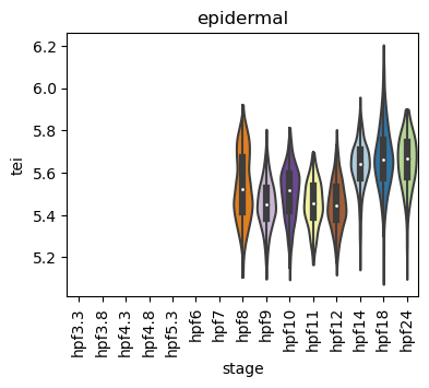
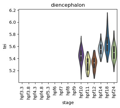
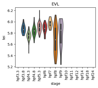
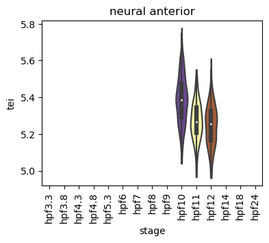
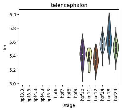
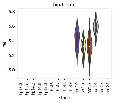
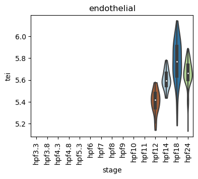
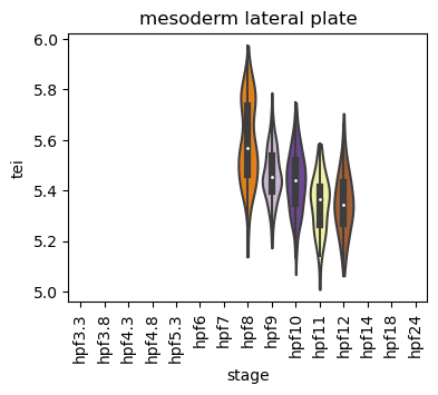
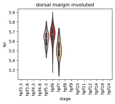
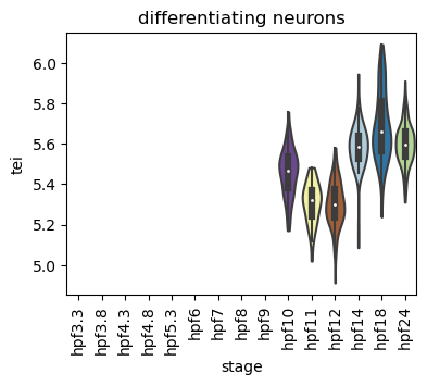
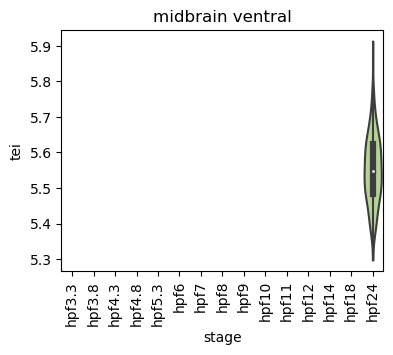
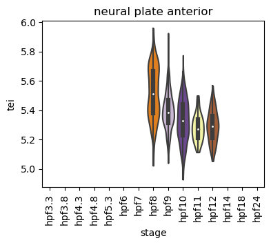
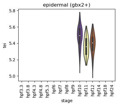
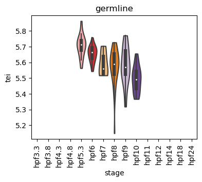
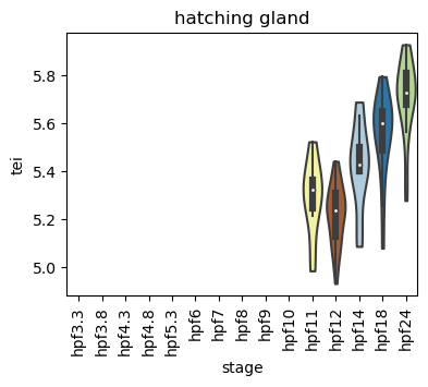
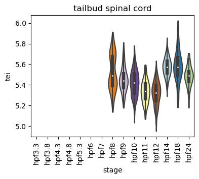
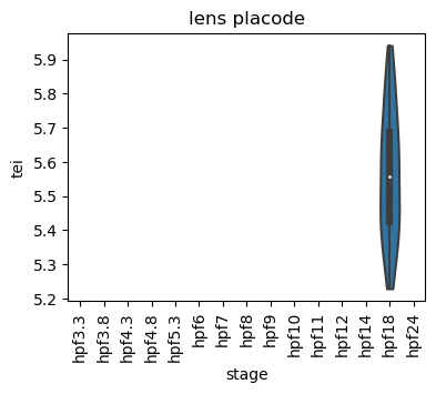
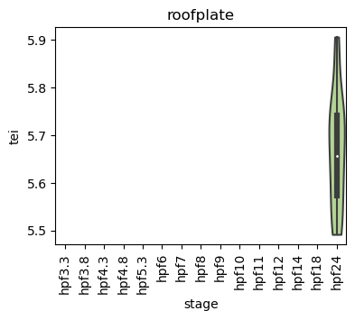
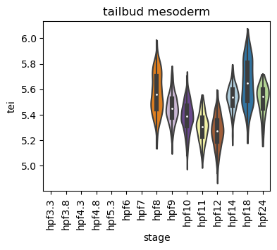
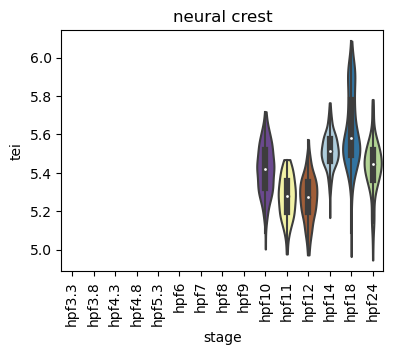
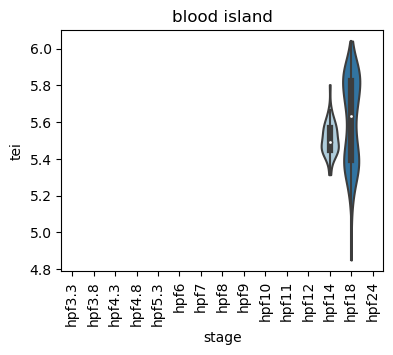
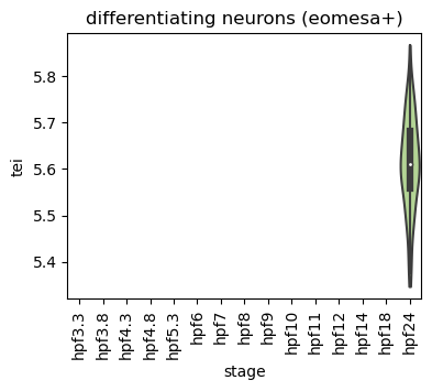
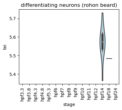
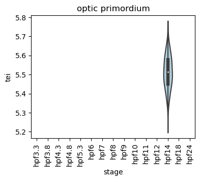
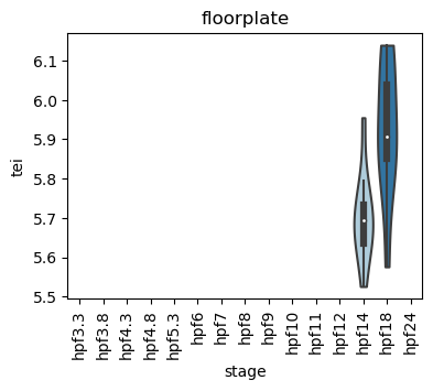
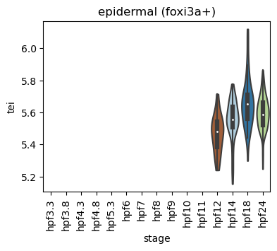
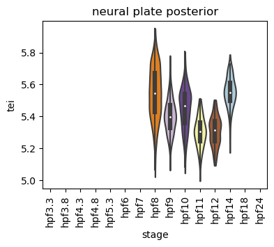
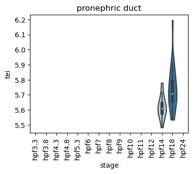
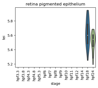
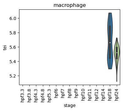
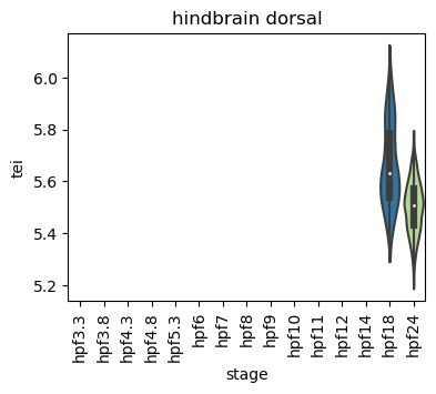
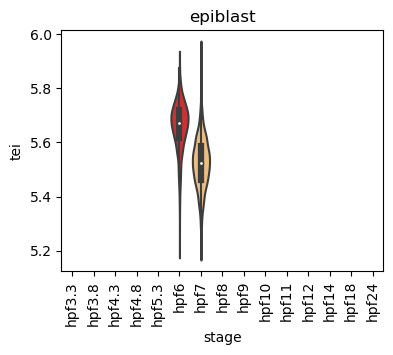
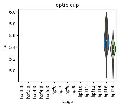
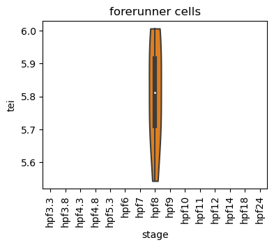
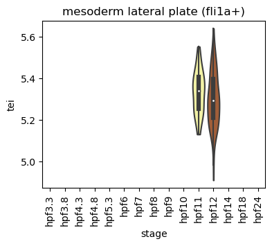
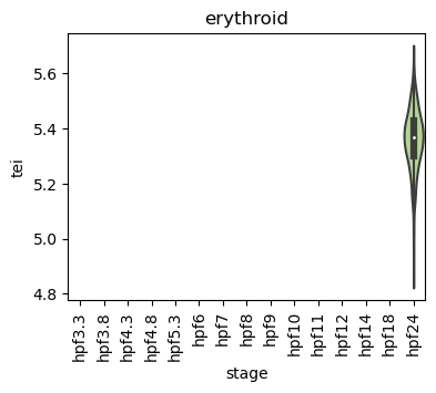
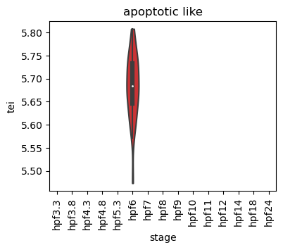
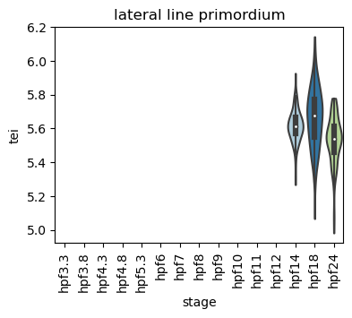
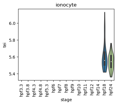
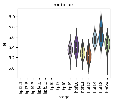
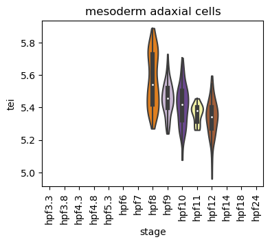
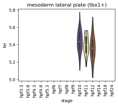
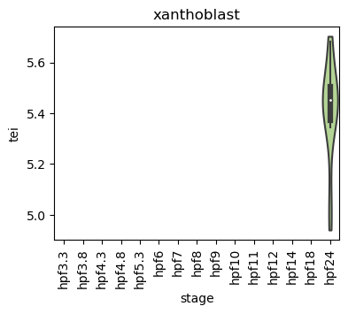
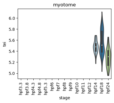
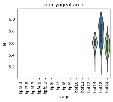
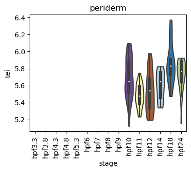
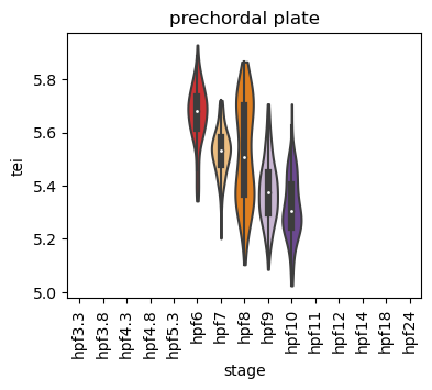
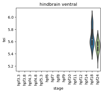
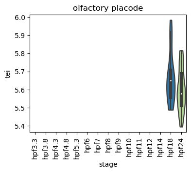
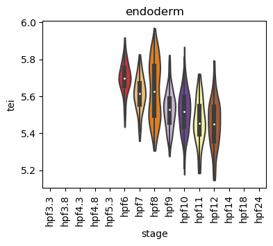
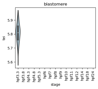
Boxplot gene age class per embryo stage and per cell type
E.g. to just show the same plot for a selected cell-type, one could do the following.
List all annotated cell types:
[26]:
list(set(zebrafish_data.obs['cell_type']))
[26]:
['DEL',
 'heart',
 'epidermal',
 'diencephalon',
 'EVL',
 'neural anterior',
 'telencephalon',
 'hindbrain',
 'endothelial',
 'mesoderm lateral plate',
 'dorsal margin involuted',
 'differentiating neurons',
 'midbrain ventral',
 'neural plate anterior',
 'epidermal (gbx2+)',
 'germline',
 'hatching gland',
 'tailbud spinal cord',
 'lens placode',
 'roofplate',
 'tailbud mesoderm',
 'neural crest',
 'blood island',
 'differentiating neurons (eomesa+)',
 'differentiating neurons (rohon beard)',
 'optic primordium',
 'floorplate',
 'epidermal (foxi3a+)',
 'neural plate posterior',
 'pronephric duct',
 'retina pigmented epithelium',
 'macrophage',
 'hindbrain dorsal',
 'epiblast',
 'optic cup',
 'forerunner cells',
 'mesoderm lateral plate (fli1a+)',
 'erythroid',
 'apoptotic like',
 'lateral line primordium',
 'ionocyte',
 'midbrain',
 'mesoderm adaxial cells',
 'mesoderm lateral plate (tbx1+)',
 'xanthoblast',
 'margin',
 'notochord',
 'pectoral fin field',
 'otic placode',
 'differentiating neurons (dlx1a+)',
 'diencephalon (aplnr2+)',
 'melanoblast',
 'non dorsal margin involuted',
 'gut',
 'myotome',
 'pharyngeal arch',
 'periderm',
 'prechordal plate',
 'hindbrain ventral',
 'olfactory placode',
 'endoderm',
 'blastomere',
 'anterior neural ridge']
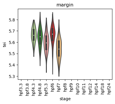
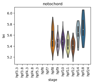
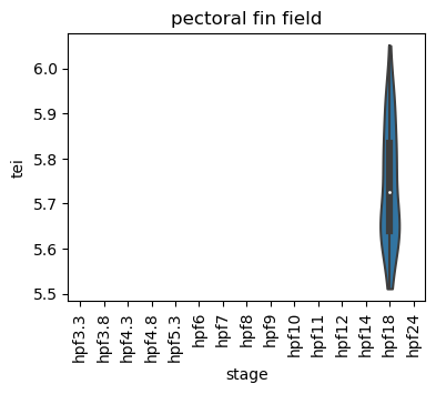
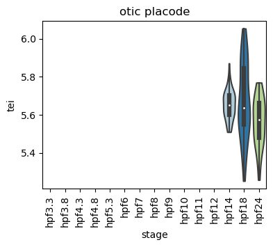
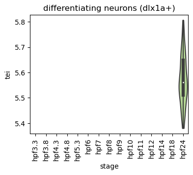
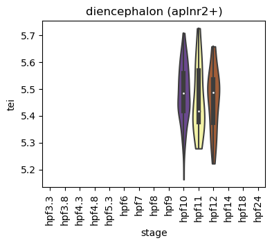
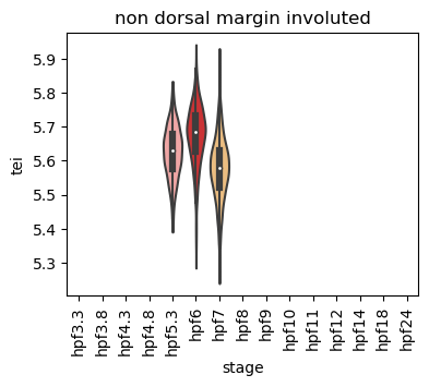
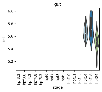
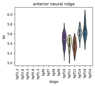
Loop over all cell types:
Note: Please change notebook cell from raw to code to see the plots.
[27]:
for ct in list(set(zebrafish_data.obs['cell_type'])):
    ax = sc.pl.violin(adata=zebrafish_data[zebrafish_data.obs['cell_type']==ct],
                      keys=['tei'],
                      groupby='stage',
                      rotation=90,
                      palette='Paired',
                      stripplot=False,
                      inner='box',
                      order=list(zebrafish_data.obs['stage'].cat.categories),
                      show=False)
    ax.set_title(ct)
    ax.set_xlabel('stage')
    plt.show()

Plot relative expression per gene age class per sample stage
[28]:
zebrafish_data_rematrix_grouped = orthomap2tei.get_rematrix(
    adata=zebrafish_data,
    gene_id=query_orthomap['geneID'],
    gene_age=query_orthomap['PSnum'],
    keep='min',
    layer=None,
    use='counts',
    var_type='mean',
    group_by_obs='stage',
    obs_fillna='__NaN',
    obs_type='mean',
    standard_scale=0,
    normalize_total=True,
    log1p=True,
    target_sum=1e6)
zebrafish_data_rematrix_grouped
[28]:
| stage | hpf3.3 | hpf3.8 | hpf4.3 | hpf4.8 | hpf5.3 | hpf6 | hpf7 | hpf8 | hpf9 | hpf10 | hpf11 | hpf12 | hpf14 | hpf18 | hpf24 |
|---|---|---|---|---|---|---|---|---|---|---|---|---|---|---|---|
| ps | |||||||||||||||
| 3 | 1.000000 | 0.763787 | 0.466752 | 0.284268 | 0.483931 | 0.481564 | 0.384060 | 0.324288 | 0.200180 | 0.263576 | 0.000000 | 0.008070 | 0.464345 | 0.564625 | 0.349337 |
| 6 | 1.000000 | 0.809081 | 0.437535 | 0.269733 | 0.388836 | 0.503856 | 0.297106 | 0.313188 | 0.155969 | 0.241321 | 0.000000 | 0.003263 | 0.499420 | 0.636556 | 0.371327 |
| 8 | 1.000000 | 0.824060 | 0.414671 | 0.254490 | 0.355464 | 0.470074 | 0.260572 | 0.288058 | 0.123445 | 0.193471 | 0.000000 | 0.003817 | 0.458995 | 0.653966 | 0.335948 |
| 10 | 1.000000 | 0.831077 | 0.411780 | 0.261339 | 0.357994 | 0.476349 | 0.260767 | 0.288836 | 0.127462 | 0.208406 | 0.000000 | 0.005533 | 0.490026 | 0.667754 | 0.351927 |
| 11 | 1.000000 | 0.865600 | 0.378906 | 0.272923 | 0.352424 | 0.471416 | 0.255806 | 0.295930 | 0.109932 | 0.183937 | 0.000000 | 0.006799 | 0.412106 | 0.616927 | 0.344885 |
| 13 | 1.000000 | 0.879969 | 0.452083 | 0.314456 | 0.410616 | 0.532115 | 0.287119 | 0.334316 | 0.129218 | 0.223298 | 0.000000 | 0.001074 | 0.544824 | 0.667480 | 0.312890 |
| 14 | 1.000000 | 0.899687 | 0.449817 | 0.328953 | 0.400997 | 0.633085 | 0.233571 | 0.321922 | 0.123774 | 0.193121 | 0.000000 | 0.000249 | 0.525102 | 0.875673 | 0.394390 |
| 16 | 1.000000 | 0.867723 | 0.548742 | 0.564756 | 0.774593 | 0.670847 | 0.604867 | 0.476988 | 0.311682 | 0.261083 | 0.048721 | 0.000000 | 0.430039 | 0.634124 | 0.286768 |
| 18 | 1.000000 | 0.869782 | 0.452952 | 0.341595 | 0.478496 | 0.249529 | 0.369100 | 0.208163 | 0.168413 | 0.066178 | 0.026141 | 0.000000 | 0.094423 | 0.185906 | 0.080072 |
| 19 | 1.000000 | 0.992605 | 0.858099 | 0.824152 | 0.884298 | 0.355240 | 0.668145 | 0.444361 | 0.441715 | 0.234261 | 0.172212 | 0.132878 | 0.091709 | 0.200682 | 0.000000 |
| 20 | 1.000000 | 0.735228 | 0.958915 | 0.727300 | 0.850712 | 0.292708 | 0.749759 | 0.473234 | 0.571193 | 0.319447 | 0.385633 | 0.362103 | 0.009518 | 0.087335 | 0.000000 |
| 22 | 1.000000 | 0.785783 | 0.241326 | 0.218616 | 0.325823 | 0.594873 | 0.328793 | 0.346191 | 0.088635 | 0.202888 | 0.000000 | 0.020581 | 0.356134 | 0.392432 | 0.033779 |
| 25 | 1.000000 | 0.998153 | 0.572311 | 0.474392 | 0.540644 | 0.265468 | 0.346071 | 0.225424 | 0.259061 | 0.147149 | 0.144565 | 0.127149 | 0.048807 | 0.176999 | 0.000000 |
| 29 | 0.925673 | 1.000000 | 0.660387 | 0.587410 | 0.709576 | 0.933434 | 0.548793 | 0.472150 | 0.218427 | 0.263950 | 0.007757 | 0.000000 | 0.364540 | 0.347877 | 0.170495 |
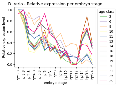
[29]:
ax = sns.lineplot(zebrafish_data_rematrix_grouped.transpose(), palette='Accent', dashes=False)
ax.legend(fontsize=5, title='age class')
ax.set_title('D. rerio - Relative expression per embryo stage')
ax.set_xlabel('embryo stage')
ax.set_ylabel('Relative expression level')
sns.move_legend(ax, 'upper left', bbox_to_anchor=(1, 1))
#plt.tick_params(labelsize=3)
plt.xticks(rotation=90)
plt.show()
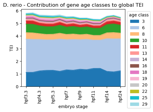
Get partial TEI values to visualize gene age class contributions
Partial TEI values can give an idea about which gene age class contributed at most to the global TEI pattern.
In detail, each gene gets a TEI contribution profile as follows:
\({TEI_{is} = f_{is} * ps_i}\)
, where \({TEI_{is}}\) is the partial TEI value of gene \({i}\), \({f_{is} = e_{is} / \sum e_{is}}\) and \({ps_i}\) is the phylostratum of gene i.
\({TEI_{is}}\) values are combined per \({ps}\).
The partial TEI values combined per strata give an overall impression of the contribution of each strata to the global TEI pattern.
One can either start from counts (adata.X) which is set as default or any other layer defined by the layer option (layer=None).
In addition, the counts can be normalized and log-transformed prior calculating partial TEI values (normalize_total=False, log1p=False, target_sum=1e6).
Further, these values can be combined per given observation, e.g. cell typer per sample timepoint (group_by='cell_state').
The get_pstrata function of the orthomap2tei submodule will return two matrix, the first contains the sum of each partial TEI per gene age class and the second the corresponding frequencies.
Both can be further processed by returning the cumsum over the gene age classes. To get them set the option cumsum=True. The cumsum will result in either for the first matrix the TEI value per cell or mean TEI value per group, if one choose a observation with the group_by option. Or in case of the second frequency matrix will result in 1.
With the standard_scale option either gene age classes (standard_scale=0 rows) or cells or groups (standard_scale=1 columns) can be scaled, subtract the minimum and divide each by its maximum. By default no scaling is applied (standard_scale=None).
The resulting data will be visualized in the downstream section.
[30]:
zebrafish_pstrata = orthomap2tei.get_pstrata(adata=zebrafish_data,
    gene_id=query_orthomap['geneID'],
    gene_age=query_orthomap['PSnum'],
    keep='min',
    layer=None,
    cumsum=False,
    group_by_obs='stage',
    obs_fillna='__NaN',
    obs_type='mean',
    standard_scale=None,
    normalize_total=True,
    log1p=True,
    target_sum=1e6)
zebrafish_pstrata[0]
[30]:
| stage | hpf3.3 | hpf3.8 | hpf4.3 | hpf4.8 | hpf5.3 | hpf6 | hpf7 | hpf8 | hpf9 | hpf10 | hpf11 | hpf12 | hpf14 | hpf18 | hpf24 |
|---|---|---|---|---|---|---|---|---|---|---|---|---|---|---|---|
| ps | |||||||||||||||
| 3 | 1.113356 | 1.114005 | 1.229654 | 1.273117 | 1.278153 | 1.197770 | 1.313577 | 1.281811 | 1.363028 | 1.330284 | 1.425889 | 1.429682 | 1.193865 | 1.152226 | 1.238431 |
| 6 | 2.637362 | 2.616733 | 2.497146 | 2.419261 | 2.424246 | 2.556530 | 2.393082 | 2.444176 | 2.345638 | 2.406803 | 2.245628 | 2.243321 | 2.590851 | 2.618168 | 2.538900 |
| 8 | 0.517103 | 0.514600 | 0.454584 | 0.430204 | 0.432281 | 0.463723 | 0.415157 | 0.429359 | 0.390495 | 0.402755 | 0.373524 | 0.373645 | 0.466532 | 0.502338 | 0.448213 |
| 10 | 0.678416 | 0.685693 | 0.622953 | 0.612870 | 0.600758 | 0.637421 | 0.585663 | 0.604837 | 0.573526 | 0.589225 | 0.571378 | 0.572683 | 0.658186 | 0.684621 | 0.636619 |
| 11 | 0.247444 | 0.254401 | 0.206657 | 0.208631 | 0.203748 | 0.221855 | 0.194637 | 0.204859 | 0.178078 | 0.185804 | 0.174756 | 0.176164 | 0.211250 | 0.230991 | 0.216543 |
| 13 | 0.135881 | 0.141672 | 0.131241 | 0.132061 | 0.128311 | 0.136144 | 0.122029 | 0.128530 | 0.116387 | 0.121953 | 0.116905 | 0.115877 | 0.140308 | 0.138097 | 0.122644 |
| 14 | 0.033937 | 0.035818 | 0.030766 | 0.030896 | 0.029582 | 0.035797 | 0.025323 | 0.028372 | 0.024326 | 0.025258 | 0.022640 | 0.022564 | 0.032801 | 0.039593 | 0.031172 |
| 16 | 0.046340 | 0.048377 | 0.051122 | 0.060191 | 0.061868 | 0.053915 | 0.060276 | 0.054464 | 0.055294 | 0.048341 | 0.050639 | 0.046917 | 0.044654 | 0.046494 | 0.043846 |
| 18 | 0.100601 | 0.104195 | 0.091349 | 0.093186 | 0.096897 | 0.068719 | 0.093560 | 0.076011 | 0.081326 | 0.064668 | 0.076974 | 0.071033 | 0.052164 | 0.054506 | 0.057179 |
| 19 | 0.094886 | 0.105762 | 0.129563 | 0.148972 | 0.135150 | 0.078638 | 0.123682 | 0.101955 | 0.116639 | 0.087341 | 0.101105 | 0.094096 | 0.050310 | 0.052783 | 0.046790 |
| 20 | 0.020965 | 0.020492 | 0.029569 | 0.030210 | 0.028496 | 0.018420 | 0.029210 | 0.025264 | 0.030754 | 0.024892 | 0.033129 | 0.032192 | 0.013354 | 0.013284 | 0.015106 |
| 22 | 0.032415 | 0.031151 | 0.021227 | 0.023941 | 0.024829 | 0.033635 | 0.027177 | 0.027644 | 0.020457 | 0.023461 | 0.020015 | 0.021431 | 0.025511 | 0.022939 | 0.014938 |
| 25 | 0.078058 | 0.088461 | 0.086041 | 0.092972 | 0.085865 | 0.061021 | 0.077996 | 0.069783 | 0.084367 | 0.071543 | 0.092356 | 0.089403 | 0.044680 | 0.047207 | 0.046444 |
| 29 | 0.068072 | 0.078519 | 0.079801 | 0.084859 | 0.085270 | 0.102441 | 0.076930 | 0.068802 | 0.049840 | 0.049623 | 0.031444 | 0.030379 | 0.052481 | 0.044994 | 0.038655 |
[31]:
#plt.rcParams['figure.figsize'] = [9, 4.5]
ax=zebrafish_pstrata[0].transpose().plot.area(cmap='tab20')
ax.legend(fontsize=3, title='age class')
ax.set_title('D. rerio - Contribution of gene age classes to global TEI')
ax.set_xlabel('embryo stage')
ax.set_ylabel('TEI')
sns.move_legend(ax, 'upper left', bbox_to_anchor=(1, 1))
plt.xticks(rotation=90)
plt.show()
#plt.rcParams['figure.figsize'] = [6, 4.5]
Gene age class contribution of one cell type
EVL:
Note: Please change notebook cell from raw to code to see the plots.
Note: Please change notebook cell from raw to code to see the plots.
hatiching gland:
Note: Please change notebook cell from raw to code to see the plots.
Note: Please change notebook cell from raw to code to see the plots.
endoderm:
Note: Please change notebook cell from raw to code to see the plots.
Note: Please change notebook cell from raw to code to see the plots.
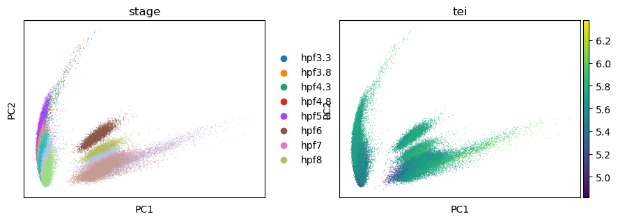
Color UMAP/TSNE by TEI
Follwoing the basic tutorial of the Scanpy python toolkit (Wolf et al., 2018), one can highlight TEI values on a dimensional reduction of the scRNA dataset, like PCA, UMAP or TSNE.
Filtering
[32]:
sc.pp.filter_genes(zebrafish_data, min_cells=3)
sc.pp.filter_cells(zebrafish_data, min_genes=200)
Normalization, Log transformation and Scaling
[33]:
sc.pp.normalize_total(zebrafish_data, target_sum=1e6)
sc.pp.log1p(zebrafish_data)
sc.pp.scale(zebrafish_data, max_value=10)
PCA and Neighbor calculations
[34]:
sc.tl.pca(zebrafish_data, svd_solver='arpack')
sc.pl.pca(zebrafish_data, color=['stage', 'tei'])
/opt/anaconda3/envs/scanpy/lib/python3.8/site-packages/scanpy/plotting/_tools/scatterplots.py:392: UserWarning: No data for colormapping provided via 'c'. Parameters 'cmap' will be ignored
  cax = scatter(
[35]:
sc.pp.neighbors(zebrafish_data)
Embedding the neighborhood graph
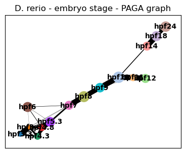
[36]:
sc.tl.paga(zebrafish_data, groups='stage')
sc.pl.paga(zebrafish_data, title='D. rerio - embryo stage - PAGA graph')
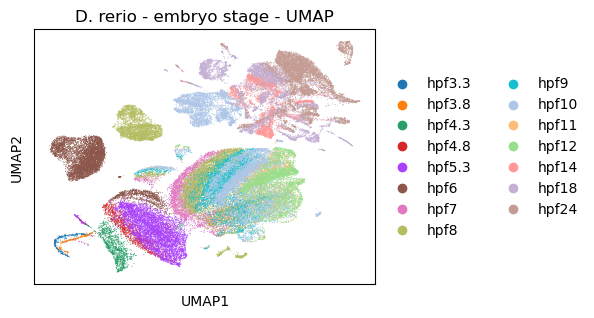
UMAP
[37]:
sc.tl.umap(zebrafish_data,
           init_pos='paga')
sc.pl.umap(zebrafish_data,
           title='D. rerio - embryo stage - UMAP', color=['stage'])
/opt/anaconda3/envs/scanpy/lib/python3.8/site-packages/scanpy/plotting/_tools/scatterplots.py:392: UserWarning: No data for colormapping provided via 'c'. Parameters 'cmap' will be ignored
  cax = scatter(
[38]:
#plt.rcParams['figure.figsize'] = [7.5, 4.5]
sc.pl.umap(zebrafish_data,
           title='D. rerio - TEI - UMAP',
           color=['tei'],
           color_map='viridis',
           vmin='p5',
           vmax='p95')
#plt.rcParams['figure.figsize'] = [6, 4.5]
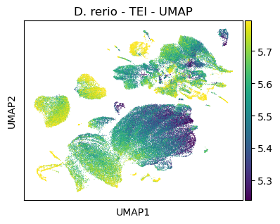
corresponds to main Figure 1F
[39]:
plt.rcParams['figure.figsize'] = [7.5, 4.5]
#3d
sc.tl.umap(zebrafish_data,
           n_components=3)
sc.pl.umap(zebrafish_data,
           title='D. rerio - embryo stage - UMAP', color=['stage'],
           projection='3d')
plt.rcParams['figure.figsize'] = [4.4, 3.3]
/opt/anaconda3/envs/scanpy/lib/python3.8/site-packages/scanpy/plotting/_tools/scatterplots.py:325: UserWarning: No data for colormapping provided via 'c'. Parameters 'cmap' will be ignored
  cax = ax.scatter(
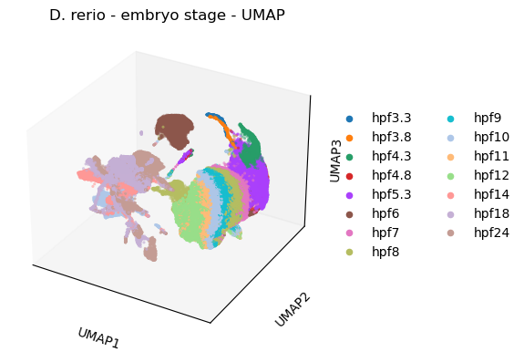
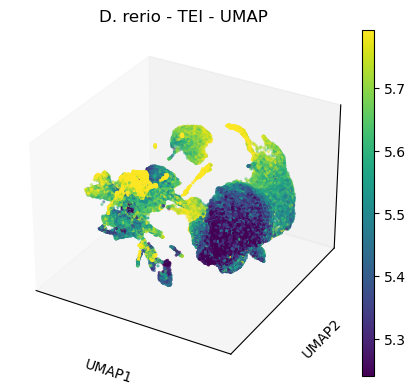
corresponds to main Figure 1G
[40]:
plt.rcParams['figure.figsize'] = [7.5, 4.5]
sc.pl.umap(zebrafish_data,
           title='D. rerio - TEI - UMAP',
           color=['tei'],
           color_map='viridis',
           vmin='p5',
           vmax='p95',
           projection='3d')
plt.rcParams['figure.figsize'] = [4.4, 3.3]
[41]:
import plotly
import kaleido
import plotly.express as px
plotly.offline.init_notebook_mode(connected=False)
[42]:
zebrafish_data
[42]:
AnnData object with n_obs × n_vars = 71203 × 19761
    obs: 'orig.ident', 'nCount_RNA', 'nFeature_RNA', 'sample', 'stage', 'group', 'cell_state', 'cell_type', 'tei', 'n_genes'
    var: 'features', 'genes', 'Phylostrata', 'n_cells', 'mean', 'std'
    uns: 'log1p', 'pca', 'stage_colors', 'neighbors', 'paga', 'stage_sizes', 'umap'
    obsm: 'X_pca', 'X_umap'
    varm: 'PCs'
    layers: 'counts'
    obsp: 'distances', 'connectivities'
[43]:
df = pd.DataFrame( {'UMAP1':zebrafish_data.obsm['X_umap'][:,0],
                    'UMAP2':zebrafish_data.obsm['X_umap'][:,1],
                    'UMAP3':zebrafish_data.obsm['X_umap'][:,2],
                    'cell_type':zebrafish_data.obs['cell_type'].values.astype(str),
                    'cell_state':zebrafish_data.obs['cell_state'].values.astype(str),
                    'tei':zebrafish_data.obs['tei'].values,
                    'stage':zebrafish_data.obs['stage'].values,
                    'cell_id':zebrafish_data.obs.index.to_list()  } )
df.set_index('cell_id', inplace = True)
df.head()
[43]:
| UMAP1 | UMAP2 | UMAP3 | cell_type | cell_state | tei | stage | |
|---|---|---|---|---|---|---|---|
| cell_id | |||||||
| hpf3.3_ZFHIGH_WT_DS5_AAAAGTTGCCTC | 8.001603 | 7.798748 | 13.366315 | blastomere | hpf3.3:blastomere | 5.847391 | hpf3.3 |
| hpf3.3_ZFHIGH_WT_DS5_AAACAAGTGTAT | 8.396315 | 7.608164 | 11.704103 | blastomere | hpf3.3:blastomere | 5.794241 | hpf3.3 |
| hpf3.3_ZFHIGH_WT_DS5_AAACACCTCGTC | 8.022252 | 7.873591 | 12.900765 | blastomere | hpf3.3:blastomere | 5.783182 | hpf3.3 |
| hpf3.3_ZFHIGH_WT_DS5_AAATGAGGTTTN | 7.795810 | 7.474202 | 14.216955 | blastomere | hpf3.3:blastomere | 5.780480 | hpf3.3 |
| hpf3.3_ZFHIGH_WT_DS5_AACCCTCTCGAT | 7.463636 | 5.477603 | 16.006929 | blastomere | hpf3.3:blastomere | 5.915213 | hpf3.3 |
[44]:
fig = px.scatter_3d(data_frame = df,
                    x='UMAP1',
                    y='UMAP2',
                    z='UMAP3',
                    color='stage')
fig.update_traces(marker_size = 2)
fig.write_html('zebrafish_scatter_3d_stage.html')
[45]:
fig = px.scatter_3d(data_frame = df,
                    x='UMAP1',
                    y='UMAP2',
                    z='UMAP3',
                    color='tei',
                    range_color=(5,5.5))
fig.update_traces(marker_size = 2)
fig.write_html('zebrafish_scatter_3d_tei.html')
[46]:
fig = px.scatter_3d(data_frame = df,
                    x='UMAP1',
                    y='UMAP2',
                    z='UMAP3',
                    color='cell_type')
fig.update_traces(marker_size = 2)
fig.write_html('zebrafish_scatter_3d_cell_type.html')
[47]:
fig = px.scatter_3d(data_frame = df,
                    x='UMAP1',
                    y='UMAP2',
                    z='UMAP3',
                    color='cell_state')
fig.update_traces(marker_size = 2)
fig.write_html('zebrafish_scatter_3d_cell_state.html')
Please have a look at the documentation for other case studies.